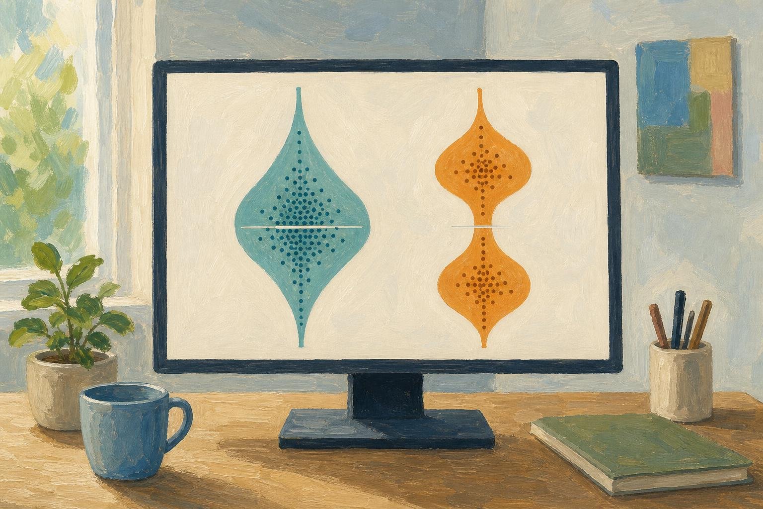
Inside a Violin Plot: Same Median, Different Shapes

Table of Contents

Two restaurants can have the same median bill while serving very different crowds: in a hypothetical example, one mostly sells $10 meals, while the other splits between $5 and $15 meals. A violin plot shows that difference by drawing a numerical distribution as a mirrored shape, wider where values are more concentrated. The useful question is what fills those bulges, so we’ll follow restaurant bills from the outline back to the individual records.

What the Shape Shows

A vertical violin has a numerical axis running through its center. Its left and right edges swell outward at values where observations concentrate, then draw inward through sparse stretches. The halves usually mirror each other; they are not separate groups. Horizontal violin charts put the numerical scale along the horizontal axis instead.

That outline usually comes from kernel density estimation, or KDE: each observation contributes a small, smooth curve, and those curves combine into an estimated distribution. Width describes concentration around a value, not the probability of observing that exact value. A cluster becomes a belly; scattered high values become a tail.

Violin plots combine that density trace with a compact statistical summary.[^history] The two layers answer different questions: where is the center, and how are values arranged around it?

[^history]: Jerry L. Hintze and Ray D. Nelson introduced violin plots in their 1998 paper, “Violin Plots: A Box Plot–Density Trace Synergism,” in The American Statistician.

Read the Axis Before the Outline

Read the labeled numerical axis first, then follow the outline along it. On a vertical bill plot, a long upper tail means a few expensive meals extend beyond the main cluster: right-skewed data. A broad lower belly places most of the concentration nearer the cheaper meals.

For a bulge that can mislead, consider invented bills clustered around cheaper and more expensive meals, with a median in the empty gap between them. Strong smoothing can blend the two clusters into one central bulge, filling a gap that the observations leave empty. The axis tells you where that invented concentration sits; the points expose it.

A violin box plot adds a box-plot summary inside the outline. Software styling varies, but displayed quartiles bracket the middle half of the observations. The median divides observations by rank. It need not sit in the widest bulge.

Use Individual Points to Judge the Shape

Points make that gap visible. A strip plot spreads observations sideways across their category; a swarm plot arranges them to reduce overlap. The sideways movement makes room for the marks, without introducing another measured variable.

Seaborn’s restaurant tips dataset supplies a real violin plot example: 244 recorded bills in US dollars and their associated tips. Each record represents a bill, not an individual diner; the separate size column records party size. Plotting total_bill shows whole-bill amounts; plotting tip shows tipping amounts. Keep that distinction in the axis label.

In the tip column, the largest observation is $10, with the next largest at $9. Overlay a swarm to show the lone $10 tip and the absence of recorded tips between those values. A smooth outline can stretch through that empty interval; individual points would make its limited support visible.

After splitting the records into smaller groups, those individual marks become especially useful. There is no universal minimum sample size for a trustworthy violin; when you can read every point comfortably, a dot plot may do the whole job.

Compare Groups on Equal Terms

For bills grouped by day, keep the dollar axis shared and the category order explicit. Calendar order answers a different reading need from an order based on typical bill size. Either can work if the arrangement is clear.

Now imagine five recorded lunch bills and fifty recorded dinner bills with the same distribution shape. Under equal-area scaling, their violins can look identical despite the tenfold difference in sample size. This is useful for comparing distributions, but the number of recorded bills needs its own label.

Equal-maximum-width scaling instead gives each group the same widest point. Count-based scaling lets relative sample sizes affect width. Choose according to the question: are you comparing the shape of spending, or should the display also communicate how many recorded bills contributed?

A split violin can place lunch on one side and dinner on the other within each day. Give the sides a clear legend and use consistent settings across subgroups. Put the bill counts beside the labels so the five-bill lunch group remains visibly a small sample.

Understand What Smoothing Changes

Bandwidth controls how broadly each observation contributes to the estimate. A small bandwidth can preserve the two clusters in the invented bills, along with minor bumps inside them. A large bandwidth can merge those clusters into one mound. More peaks do not necessarily mean more populations.

Use the points to distinguish a persistent gap from a ripple in the estimate. If a suspected second peak survives reasonable bandwidth changes and has observations clustered beneath it, you have a stronger reason to investigate what separates those bills.

Smoothing also reaches beyond individual observations. In seaborn, cut=0 stops the displayed density at the observed minimum and maximum; it clips the drawing without correcting boundary bias in the estimate. Without a range restriction, a smooth kernel can carry a positive-valued bill distribution below zero, drawing a tail of negative restaurant tabs.

Build a Plot With Explicit Settings

For the tips data, begin with a specific comparison: how do bill distributions differ by day? This example requires seaborn 0.13.0 or later. Install the packages from a terminal:

python -m pip install "seaborn>=0.13.0" matplotlib

Then run the Python block below. Loading the example dataset requires internet access unless it is already cached locally.

import seaborn as sns
import matplotlib.pyplot as plt

tips = sns.load_dataset("tips")

sns.violinplot(
    data=tips,
    x="day",
    y="total_bill",
    inner="quart",
    cut=0,
    density_norm="area",
    bw_adjust=1,
)

plt.show()

This call draws a separate vertical silhouette at each day category, with bill amounts on the vertical axis and quartile marks inside. Each silhouette ends at its group's observed bill limits. Area-based density scaling compares concentration rather than bill counts. With cut=0, clipping can leave different visible areas: seaborn does not renormalize the remaining area after clipping.

Add the label “Total bill (US dollars)” to make the units explicit. Pair the plot with bill counts and, where legible, overlaid observations. A useful caption names the area-based density scaling, clipping at observed limits, and bandwidth adjustment; it gives readers the choices behind the outline without explaining every argument in the call.

Key Takeaways

Read the numerical axis before interpreting a bulge or tail.
Use internal summary marks to locate the center, and points to see what supports the outline.
Match width scaling to the comparison: distribution shape or relative sample size.
Treat a peak as a feature to investigate, especially when smoothing changes it.

Frequently Asked Questions

What is the difference between a boxplot and a violin plot?

A boxplot shows a compact summary, usually a median, quartiles, and rule-defined whiskers; a violin adds an estimated density outline. Two groups can share those boxplot summaries yet arrange their observations differently between the marks, which the outline can reveal.

How do I create a violin plot?

To create a violin plot, choose a numerical column, assign any grouping column, and draw its density with explicit smoothing and scaling settings. The Python example above supplies those settings; R's ggplot2 offers geom_violin(), and MATLAB offers violinplot, though defaults and styling differ.

Are violin plots good?

Violin plots are useful when the shape of a distribution matters to your comparison. If your question is the exact amount of each recorded bill, individual points answer it more directly than a smooth silhouette.

Can I do a violin plot in Excel?

You can make a violin plot in Excel using calculated density values and a custom chart arrangement, or an add-in, but Excel has no native violin chart type. Its built-in Box and Whisker chart is simpler when a density outline adds little to your decision.

Why does changing the bandwidth change the apparent number of peaks?

Changing the bandwidth changes how strongly neighboring observations blend together. Closely spaced clusters may remain separate under narrow smoothing and join under broad smoothing, so the apparent number of peaks belongs partly to the estimate.

Read the Shape, Check the Data

Choose the display by the decision you need to make. If you are comparing spending patterns across days, begin with bills on one shared dollar scale and keep the observations available beside the density. If you need to identify a particular expensive meal, use the records or a dot plot instead.

The decisive feature is sometimes an absence: the invented bills have a median in a gap without a single purchase at that value. That gap is information, even when smoothing fills it. Let the violin reveal a pattern worth examining, then let the observations determine how you describe it. A useful chart makes the distinction between a measured value and an estimated shape easy to see.