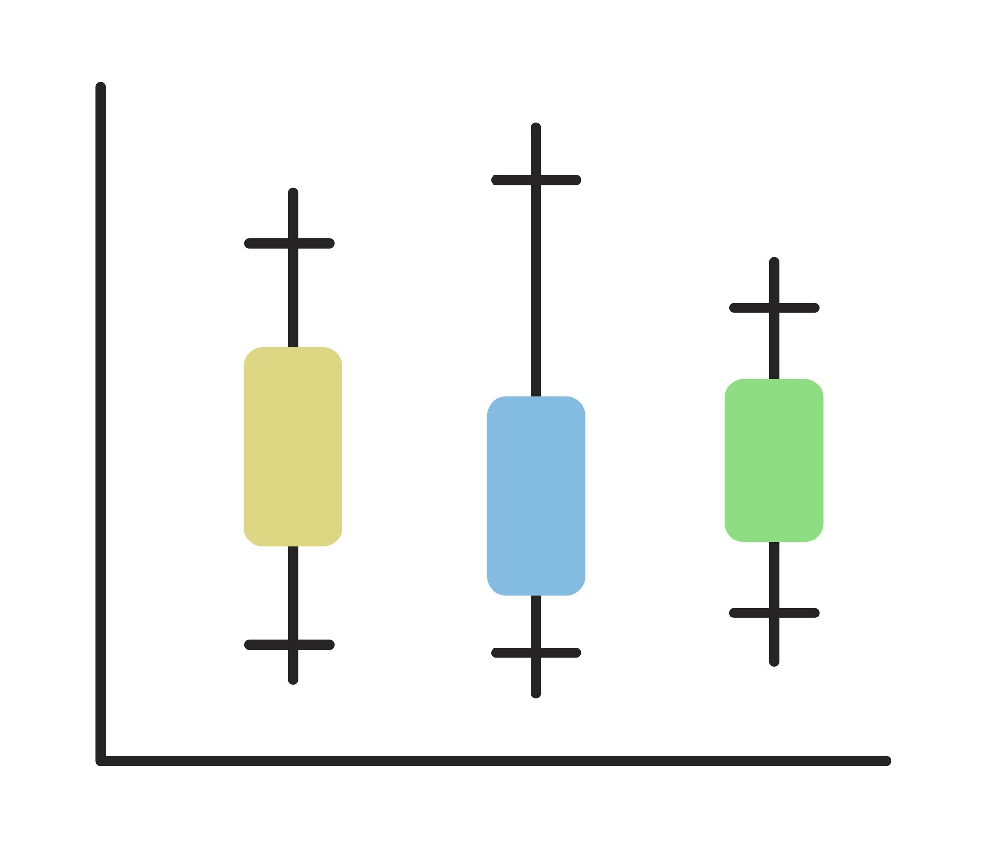
A box plot summarizes a dataset’s center and spread using a median line, a box, and whiskers. A shorter box can belong to a slower team: in a chart of task completion times, a tight cluster of longer times means consistency, not speed.

That distinction matters when you compare box plots. Read each display as an answer to a practical question: where does a typical result fall, and how much do results vary around it? The task-time examples below put those two questions on the same scale.

In This Article

• Read the Box, Line, and Axis
• Work Through a Small Example
• Understand Where the Whiskers Stop
• Look for Asymmetry Without Assuming the Shape
• Compare Groups on the Same Scale
• Know What the Summary Leaves Out
• Key Takeaways
• Frequently Asked Questions
• Start With the Median and Spread

Read the Box, Line, and Axis

The measurement axis gives the box its meaning. A horizontal chart places values along the horizontal axis; a vertical chart places them along the vertical axis. Higher on the page means a larger measurement only when the value axis runs upward. An axis labeled in minutes turns distance along that scale into a difference in completion time.

On that scale, the box stretches from the first quartile, Q1, to the third quartile, Q3. These mark the 25th and 75th percentiles, enclosing the middle 50% of observations. The box’s length therefore describes how widely the central results spread. Ties can put several observations on a boundary, so those percentages describe rank positions rather than four necessarily equal-sized piles.

Inside the box, a line marks the median, Q2: the central value after the observations are ordered. Its position tells you where the typical result sits; its distance from either edge shows how the two halves of the box occupy the measurement scale. A separate, labeled symbol may also show the mean, offering another measure of center.

Work Through a Small Example

For a box plot example, suppose ten hypothetical task completion times, in minutes, are already sorted:

2, 4, 5, 6, 8, 9, 11, 12, 14, 30.

The two central values are 8 and 9. Their average gives a median of 8.5 minutes, placing the median line between two observed times. Nobody needs to have completed the task in exactly that time for it to be the center of the ordered results.

Use the median-of-halves method to find the box edges. The middle value of the lower five observations gives Q1 = 5 minutes; the middle value of the upper five gives Q3 = 12 minutes. Subtracting Q1 from Q3 gives the interquartile range, or IQR: 12 − 5 = 7 minutes.

The box now has a concrete meaning: its edges mark the middle half of the ordered results. The mean is 10.1 minutes, compared with the median of 8.5 minutes. The largest time pulls the mean upward, giving two different answers to what a “typical” completion time might mean.

Understand Where the Whiskers Stop

The 30-minute result also explains why a whisker may stop short of the largest observation. Under a common convention, whiskers reach the most extreme observed values within two calculated limits:

• Lower fence: Q1 − 1.5 × IQR
• Upper fence: Q3 + 1.5 × IQR

An IQR box plot uses these fences to separate the whiskers from individually plotted points. A fence is a threshold; a whisker endpoint is an observation. That distinction explains why the two usually occupy different positions.

For the task times, the lower fence is 5 − 1.5 × 7 = −5.5 minutes; the upper fence is 12 + 1.5 × 7 = 22.5 minutes. The whiskers end at 2 and 14 minutes, the outermost observations within those limits. The negative lower fence is an arithmetic threshold, not a negative completion time. The 30-minute observation exceeds 22.5 and appears separately.

That point invites a practical question. Was the task interrupted, or did this case genuinely take much longer? Either explanation is possible in this hypothetical example. Investigate its context before deciding how to analyze it; the outlier flag alone supplies no reason to delete it.

Look for Asymmetry Without Assuming the Shape

The example’s full display leans toward longer times. The separate point stretches the upper-value tail all the way to 30. Judging only the whisker lengths would miss the strongest feature.

That extended upper tail suggests right skew, consistent with the mean sitting above the median. “Right” describes the direction toward larger values: on a vertical chart, the same tail points upward. A longer lower-value tail would instead suggest left skew.

The median’s position adds a different clue. When it sits closer to Q1 than Q3, the upper half of the box spans a wider numerical interval. The observations in that half are more spread out, not more numerous. Read the median’s position alongside the tails: the box and the distant high point tell different parts of the story.

Compare Groups on the Same Scale

Suppose you must choose between two hypothetical teams for a task. The first has the worked example’s ten results. The second also has ten times, in minutes: 5, 8, 9, 10, 11, 11, 12, 13, 14, 17. Using the same method, its median is 11, Q1 is 9, Q3 is 13, and IQR is 4 minutes. Its fences are 3 and 19 minutes, so its whiskers end at 5 and 17, with no outliers. Put both on one minutes axis and label each sample size as n = 10. Separately scaled panels could make their box lengths look alike and conceal the difference you need to judge.

On that common scale, the second team is slower at the center but more consistent across its central results. For work where typical turnaround drives the decision, the first team has the advantage. For scheduling work into predictable time slots, the second team’s tighter central spread may be attractive. Its narrower box does not, however, establish how often it misses a particular deadline; that question needs the actual times near and beyond the cutoff.

The number of observations also affects how firmly to hold that comparison. A box based on fewer observations can shift substantially when a few new results arrive. A box based on more observations usually gives a more stable summary under comparable sampling conditions. Standard box widths often do not represent sample size, although some variable-width designs do. Give a sparsely supported comparison less weight when choosing how to run the work.

Know What the Summary Leaves Out

A deadline decision can turn on details that quartiles hide. Consider these two hypothetical sets of completion times, using the same median-of-halves method:

• Clustered times: 0, 1, 2, 2, 2, 2, 8, 8, 8, 8, 9, 10.
• More evenly spread times: 0, 1, 2, 2, 4, 5, 5, 6, 8, 8, 9, 10.

Both have matching quartiles and whisker endpoints under the fence rule above. Their standard box plots are identical.

Their working patterns are not. The first set is more clustered; the second is more evenly spread. A manager planning around a five-minute task would face a different pattern in each case, despite seeing the same median line.

A dot plot exposes those individual values; a histogram shows where observations accumulate. Overlaying points is especially useful for small samples like these. The extra view answers a question the box cannot: are results gathered around distinct times, or spread through the interval?

Key Takeaways

• Use the median to compare typical results, and the box length to compare central consistency.
• Include separate points when judging which way a tail extends.
• Treat an outlier flag as a reason to investigate the observation’s context.
• Choose between speed and consistency according to the work the chart represents.
• Add individual values when clusters or a deadline could change the decision.

Frequently Asked Questions

What Is a Box Plot?

A box plot, also spelled “boxplot” and called a “box and whiskers plot”, is a compact chart of a numerical dataset’s median, quartiles, and tails. It makes differences in center and spread easy to compare across groups. Quartile and whisker definitions can vary between displays.

Can You Tell Whether a Distribution Is Normal From a Box Plot?

A box plot cannot establish whether a distribution is normal. A balanced-looking box can hide different shapes, so use a histogram and, when normality matters to an analysis, a normal probability plot or Q–Q plot.

How Do You Find Q1, Q2, and Q3 in a Box Plot?

Read Q1 and Q3 at the box’s two ends along the value axis, and Q2 at the median line inside it. For raw data, order the values and use a specified quartile method, such as the median-of-halves method used here.

What Are Outliers in a Box and Whisker Plot?

Under the common 1.5 × IQR rule, outliers are observations beyond the lower or upper fence, usually drawn as separate points. The label describes their distance from the central data, not whether they are valid observations.

Do Whiskers Always Extend to the Minimum and Maximum?

Whiskers do not always extend to the minimum and maximum: IQR-based whiskers stop at the outermost observations within the fences. Other conventions use the full observed range or specified percentiles, so whisker definitions vary between displays.

Start With the Median and Spread

Choose the question before choosing the team. If typical turnaround matters most, favor the lower median; if predictable central results matter more, give the narrower box more weight. In the task-time comparison, those priorities favor different groups. A deadline calls for a closer look at the observations themselves, especially the long completion times.

That closer look is worth taking whenever a decision rests on the clean summary. The two sets with matching quartiles showed why: their working patterns differed. Keep the box as a useful compression of the data. The individual observations can change the decision even when the box stays the same.