
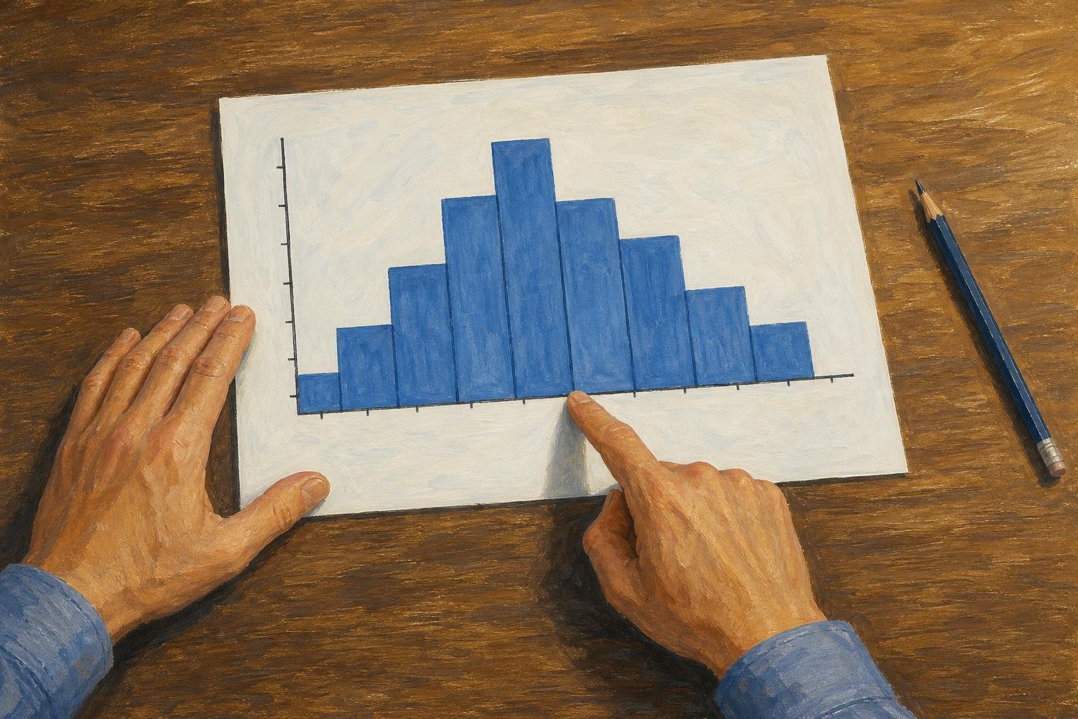

A histogram shows how numerical observations fall into intervals: each bar represents a range, and its height or area tells you how much data falls there. Learning how to read a histogram means checking the axes first, then interpreting the bars according to the vertical scale.
The reading order is consistent: identify the measurement, establish what each bar represents, and then describe the distribution. The sections below use an illustrative set of book lengths to explain counts, proportions, and the limits of grouped data. A separate example shows why unequal bin widths require attention to area.
In This Article
- Read the Axes Before Comparing Bars
- Follow the Interval Boundaries
- Turn Bar Counts Into Answers
- Locate the Middle Without Inventing Precision
- Describe the Pattern and Its Limits
- Use Area When Bin Widths Differ
- Key Takeaways
- Frequently Asked Questions
- What a Histogram Reveals and What Remains Unknown
Read the Axes Before Comparing Bars
The horizontal axis identifies the numerical variable and its units. For book lengths, that might be “Number of pages,” with intervals running from 100 to 350 pages. The vertical axis tells you whether the bars show counts, percentages, or density. A height of 20 could therefore mean 20 books, 20% of the books, or a density value. The label decides.
Learning how to read a histogram starts with that numerical axis, which separates it from a bar chart. A histogram groups observations into ordered intervals; a bar chart compares categories, such as fiction, biography, and poetry. You can rearrange those categories without changing their meaning, but moving numerical intervals out of order would misrepresent the measurement. Adjacent histogram bins touch because their intervals meet. An empty interval represents zero observations.
Follow the Interval Boundaries
Intervals, also called bins, need a rule for observations that land on a boundary. One common convention includes the lower boundary and excludes the upper one. Under that rule, a bin labeled 150–200 contains books with at least 150 pages but fewer than 200. A book with exactly 200 pages belongs in the next bin.
That boundary rule ensures each observation is counted once. Chart notes or interval notation may specify a different convention, especially for the final endpoint. The notation [150, 200), for example, explicitly includes 150 and excludes 200.
Boundaries also limit what you can recover. If a bin covers 200–250 pages, its bar does not reveal how many books have fewer than 225 pages. The observations could cluster near either end. Dividing the count in half assumes that half the observations fall on each side of 225.
Turn Bar Counts Into Answers
Consider an illustrative collection of 50 books divided into equal-width, 50-page bins. The counts are 5 for 100–150 pages, 15 for 150–200, 20 for 200–250, 8 for 250–300, and 2 for 300–350. These counts add to the stated total, which gives you a denominator for calculating proportions.
The worked example can organize which questions require a single bar and which require combining bars:
How to read a histogram: counts and proportions for 50 books
| Book-length question | Histogram bins to use | Count out of 50 books | Proportion of books | Reading method |
|---|---|---|---|---|
| 200 ≤ pages < 250 | 200–250: 20 | 20 | 20 ÷ 50 = 40% | Read one bar |
| 150 ≤ pages < 250 | 150–200: 15; 200–250: 20 | 15 + 20 = 35 | 35 ÷ 50 = 70% | Add two adjacent bars |
| Fewer than 200 pages | 100–150: 5; 150–200: 15 | 5 + 15 = 20 | 20 ÷ 50 = 40% | Sum bins below the cutoff |
| At least 250 pages | 250–300: 8; 300–350: 2 | 8 + 2 = 10 | 10 ÷ 50 = 20% | Sum bins at or above the cutoff |
| At least 300 pages | 300–350: 2 | 2 | 2 ÷ 50 = 4% | Read the final bar |
| Fewer than 225 pages | 20 below 200; 20 in the 200–250 bin | 20–40; exact count unknown | 40%–80%; exact proportion unknown | Cutoff splits a bin; only bounds are known |
For the proportion of books from 150 up to 250 pages, add the two relevant counts: 15 + 20 = 35. Then divide by the total: 35 ÷ 50 = 0.70, or 70%. This calculation works exactly because the requested range follows bin boundaries.
Those boundaries matter when wording the result. Saying “between 150 and 250 pages” can leave endpoint inclusion unclear; “at least 150 but fewer than 250 pages” matches the convention established above. Exact wording prevents a correct calculation from becoming an ambiguous claim.
Locate the Middle Without Inventing Precision
The tallest frequency bar identifies the modal interval: the interval containing the most observations. In the book example, 200–250 pages is the modal interval. The most-common individual page count remains unknown.
To locate the median, accumulate counts from the left. For an odd number of observations, find the bin containing the single middle observation. For an even number, locate both middle observations: the median is their average. They can fall in different bins, so there may be no single bin containing both, and their average can lie between those bins.
For the 50 books, cumulative counts are 5, 20, 40, 48, and 50. The 25th and 26th observations both fall in 200 ≤ pages < 250, so the median is in that interval. Its exact value remains unknown.
An estimated mean requires an additional assumption. Using each bin’s midpoint as a stand-in for its observations gives a weighted total of 10,600 pages; dividing by the collection size gives an estimated mean of 212 pages. That estimate treats every book within a bin as if it had the midpoint page count. The actual mean could differ.
Describe the Pattern and Its Limits
Check the overall pattern: roughly matching sides suggest symmetry, roughly equal heights across equal-width bins suggest uniformity, and a longer tail names the direction of skew. The occupied bins show the approximate spread; in the book example, the exact shortest and longest books remain unknown.
Keep descriptions tied to the displayed bins. Wider bins can merge clusters, while narrower bins can produce an irregular outline. An isolated bar deserves a closer look at the underlying observations before you classify them as errors or valid unusual cases.
Use Area When Bin Widths Differ
Unequal-width bins change how you compare bars. For a frequency-density histogram, frequency density = count ÷ bin width. Rearranging gives count = bar height × bin width. Compare bar areas to compare frequencies.
For a separate illustrative dataset, suppose 12 observations occupy an interval from 0 to 10, while 18 occupy an interval from 10 to 30. Their widths are 10 and 20, so their frequency densities are 1.2 and 0.9. The first bar is taller despite containing fewer observations. Multiplying each height by its width recovers the counts.
Probability density uses the same area principle but represents proportions. For this dataset, the corresponding heights are 0.04 and 0.03. Their areas are 0.4 and 0.6, and the total bar area is 1. A probability-density height is not itself the probability of falling within that interval.
Key Takeaways
- The variable, units, bin boundaries, and vertical scale establish what the bars represent.
- The tallest frequency bar identifies the interval containing the most observations.
- Combined bin counts divided by the total give the proportion within those intervals.
- A histogram reveals approximate center, spread, and visible pattern, but grouping limits precision.
- Bin widths and grouping affect comparisons of bar heights and the conclusions they support.
Frequently Asked Questions
How Can I Tell the Mean and Median From a Histogram?
Estimate the mean by multiplying each bin midpoint by its count, adding those products, and dividing by the total count. For the median, use cumulative counts to locate the middle observation in an odd-sized sample or both middle observations in an even-sized sample. Those two observations may occupy different bins; their average is the median. Grouped data generally do not reveal either summary exactly.
What Should a Correct Histogram Look Like?
It should have labeled numerical intervals, a clearly identified vertical scale, and bars whose heights or areas correctly represent the data. Adjacent intervals meet; a zero-count interval remains empty. There is no required overall shape: a correct histogram need not resemble a bell.
What Are the Rules of a Histogram?
Bins must not overlap, and each included observation must belong to exactly one bin. Numerical intervals stay in order, with their widths represented accurately. When widths differ, use an appropriate density scale so that bar area represents count or proportion.
Can a Histogram Show the Exact Number of Observations Below a Value Inside a Bin?
Usually, no: it gives the count for the whole interval, not the positions of observations within it. You can total the completed bins below that value, but the partial bin introduces uncertainty. An exact answer requires the underlying data or additional information.
Why Can Two Histograms of the Same Data Look Different?
Different bin widths or starting boundaries can split and combine the same observations differently. One chart may also use counts while another uses percentages or density. Compare those construction choices before treating the outlines as conflicting evidence.
What a Histogram Reveals and What Remains Unknown
A histogram shows how observations are distributed across numerical intervals. The resulting pattern reveals center, spread, and shape, although bin choices affect what is visible.
The chart’s grouping limits the precision of its answers. In the book example, exactly 70% have at least 150 but fewer than 250 pages because those cutoffs follow bin boundaries. The proportion below 225 pages is only bounded between 40% and 80%, because that cutoff splits a bin. Likewise, the midpoint-based mean of 212 pages is an estimate, not an exact result.
Recommended for you

Area Chart Fill: Separate Values or a Shared Total?
An area chart uses fill to emphasize magnitude, but stacked and separate values mean different things. See the distinctions and learn how to build one in Excel.

The Visual Language of Books: How Covers Communicate Complexity
At thumbnail size—often 100–160 pixels wide on retail grids—a cover must communicate genre, tone, and complexity before a reader can zoom in. The difference between a muddled thumbnail and a crisp focal point can determine whether a title gets a click, a pickup, or a pass. If you want a practical method for turning ideas […]
Mapped: How a Bill Becomes a Law Flowchart—Key Decisions
Use this how a bill becomes a law flowchart to trace committee review, chamber votes and presidential action. See why bills move forward or stop along the way.
Math Line Plot: Each Mark a Measurement, Each Stack a Count
A line plot turns nine bean pod lengths into visible counts. Learn what marks and stacks mean, then build your own with fractions. See the worked example.
Box Plot Reading: A Shorter Box Doesn’t Mean Faster
A box plot shows center and spread, not speed alone. Use task-time examples to compare medians and variability on the same scale. See the worked example.
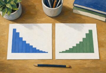
Right vs Left Skewed Histogram: What the Tail Reveals
A right vs left skewed histogram is named for its tail, not its tallest bars. Avoid reversed readings and check averages and binning. Explore the guide.

Stacked Bar Chart: Totals, Parts, and Shares Made Clear
A stacked bar chart shows totals and the parts behind them. Learn when to use counts or percentages, with a worked example and Excel steps. See the guide.
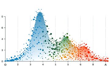
Bimodal Histogram: Two Peaks That One Average Can Hide
A bimodal histogram can reveal two operating conditions. Use the 15 and 25 millisecond test example to read the peaks and plan your next analysis. See how.