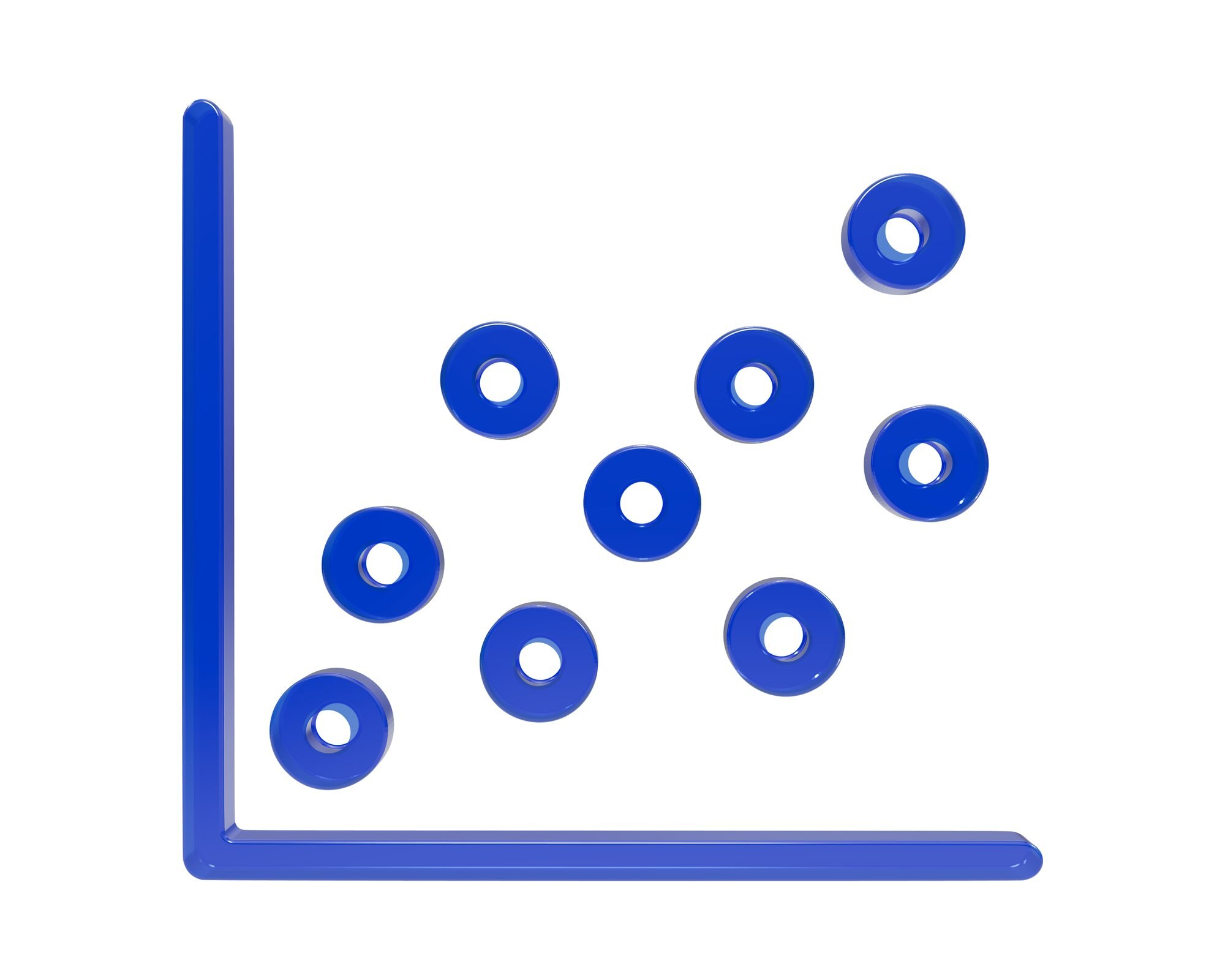
A scatter plot shows the relationship between two numerical variables, with each dot representing one observation’s paired values. A steep upward cloud can look persuasive even when its points are widely scattered: the angle catches your eye, but the scatter tells you how consistent the relationship is.

Reading that difference is the task. The sections below move from individual dots to the overall pattern, then examine what grouping and display choices reveal or hide.

In This Article

• Start With the Right Variable Pair
• Read the Axes and Identify Each Dot
• Look for Direction and Shape
• Judge Strength With a Trend Line and Correlation
• Examine Clusters and Unusual Points
• Watch for Display Choices That Change the Picture
• Use Color and Size Only When They Help
• Key Takeaways
• Frequently Asked Questions
• What a Scatter Plot Reveals

Start With the Right Variable Pair

Frame the vehicle question narrowly: “Among comparable vehicles, how does fuel economy vary with horsepower?” That wording identifies the variable pair and makes the comparison group explicit.

A useful reading might be: “Across all vehicles, higher horsepower generally accompanies lower fuel economy, but the pattern is weaker within each vehicle class.” Use that qualification only if the plotted groups support it. It tells the reader more than a single description of the combined cloud.

Read the Axes and Identify Each Dot

Suppose a dot represents a hypothetical truck with 450 horsepower and fuel economy of 12 miles per gallon. With horsepower on the horizontal x-axis and fuel economy on the vertical y-axis, that truck sits at (450, 12). Each coordinate belongs to the same vehicle; scatter plot data cannot be assembled meaningfully from two unrelated lists.

Read the units as carefully as the names. Also inspect the scale: on a logarithmic axis, equal distances represent equal ratios, not equal differences. The x-axis often carries the explanatory variable and the y-axis the response variable, expressing the question being asked.

For the truck, the dot is one vehicle with two measurements. It is not a count of 450 trucks.

Look for Direction and Shape

Follow the cloud from left to right. Rising points indicate positive association; falling points indicate negative association. Temperature and ice cream sales are familiar scatter plot examples for an upward pattern, while horsepower and fuel economy illustrate a question where you might expect a downward one.

In a positive scatter plot, larger x-values tend to accompany larger y-values. Shape adds another piece: a linear scatter plot forms an approximately straight band, whether it rises or falls.

A curve tells a different story. Imagine plotting outdoor temperature against a building’s energy use: high use on cold days for heating, low use at mild temperatures, then high use on hot days for cooling. That hypothetical U-shape has a clear pattern without one overall upward or downward direction. A cloud with neither direction nor another recognizable shape has little visible association.

Judge Strength With a Trend Line and Correlation

Strength means closeness to the pattern. A narrow diagonal band shows a stronger linear association than a broad cloud, even if the broad cloud looks steeper. Slope describes the tilt; spread describes the consistency.

A fitted trend line gives you a reference through that cloud. An isolated point far to the right can pull the fitted line toward itself, changing the apparent tendency across the chart. Compare the line with the main group, not merely with the most conspicuous dot. Extending it beyond the observed range adds assumptions the plotted measurements cannot support.

Pearson’s correlation coefficient, r, summarizes linear association and ranges from −1 to +1. Its sign gives direction: −1 indicates a perfect negative linear relationship, and +1 a perfect positive one. Values closer to either endpoint indicate stronger linear association; zero means no linear association, not necessarily no relationship. A value near zero can accompany the U-shaped example above. Read the shape before accepting the summary.

Examine Clusters and Unusual Points

Suppose the vehicle chart contains two clusters: small gasoline hatchbacks and heavy diesel pickups. The combined cloud might slope downward mainly because the pickups occupy the high-horsepower, low-economy corner. Separate the groups and ask whether horsepower still tracks fuel economy within each one.

That split brings vehicle weight into the question. Weight could help explain the overall pattern, and the two-variable display cannot isolate its contribution. An association across all vehicles can weaken or reverse when groups are separated; the chart alone does not establish cause and effect.

An outlier poses a more local question. It might sit far along the x-axis or far above the surrounding pattern. Consider its measurement and context, then compare the analysis with and without it. One unusual truck could be the observation holding the fitted slope in place.

Watch for Display Choices That Change the Picture

Axis ranges and chart proportions can make the same cloud look steep or flat. Read labeled values instead of judging the angle alone. Scatter plot axes need not begin at zero, although a tightly cropped range can magnify small differences.

Overlapping markers create another distortion: several observations at the same coordinates can look like one. Smaller markers reduce crowding, while transparency makes heavily overlapping areas darker, revealing density that opaque dots conceal.

Jitter separates coincident markers by adding small display offsets, especially for rounded or discrete measurements. Label that adjustment because the displaced positions are not measured values. A single crowded dot becomes a small spray of points.

Use Color and Size Only When They Help

Color can expose the hatchback–pickup split without changing either axis. A clear legend lets you compare each group’s pattern before reading the combined cloud. Point size can encode another numerical variable, producing a bubble chart; when size represents quantity, bubble area should scale with it.

Now imagine that vehicle weight controls bubble size and the heaviest vehicles become giant opaque discs. Those discs cover smaller cars and obscure the very groups the colors were meant to distinguish. Bigger does not mean more reliable unless reliability is explicitly the size variable.

If your question is simply how many vehicles belong to each class, use a bar chart for those category totals. A bubble chart full of overlapping discs makes that count needlessly hard to read.

Key Takeaways

• Establish what one dot represents before interpreting the cloud.
• Describe the shape before using a straight-line summary.
• Compare group patterns with the combined pattern.
• Investigate an influential point instead of silently deleting it.
• Treat marker overlap as missing visual information, not missing observations.

Frequently Asked Questions

What is a scatter plot used for?

A scatter plot is used to examine relationships between paired numerical measurements and identify influential observations. A concrete example is statistician Francis Anscombe’s fourth demonstration dataset, published in 1973: one point with an unusual x-value determines the fitted slope, while the remaining points share one x-value. It shows how a numerical summary can encourage a trend-based interpretation that the plotted observations undermine.

How do I make a scatter plot?

Put one observation in each row, place its two numerical measurements in separate columns, and select those columns to create a scatter chart in your software. Label both axes with names and units so a coordinate has a clear meaning. If a vehicle’s fuel-economy measurement is missing, leave it missing instead of inserting zero unless zero is its actual value.

How do you interpret a scatter plot?

Interpret a scatter plot by describing its overall pattern and the observations that depart from it. For the vehicle example, a useful statement is “higher horsepower generally accompanies lower miles per gallon in this dataset.” If colors reveal separate vehicle classes, add whether that tendency appears within the classes or only across them.

What are the three types of scatter plots?

Three common introductory patterns are positive association, negative association, and no apparent association. The temperature–energy example is U-shaped, not an example of no association.

Does one outlier mean the relationship should be ignored?

No; one outlier means you should examine how heavily the conclusion depends on that observation. Compare the fitted result with and without it, and report a major change. Remove the point only for a defensible reason, such as a documented recording error.

What a Scatter Plot Reveals

A scatter plot shows how paired numerical measurements vary together. Each dot contributes to a pattern whose direction, shape, and strength matter more than its apparent steepness. Groups and unusual observations can change what a fitted line or correlation suggests, while axis scales and overlapping markers affect what is visible.

The resulting interpretation has limits as well as a pattern. In the vehicle example, a tendency across all vehicles does not necessarily describe the relationship within comparable classes, and neither pattern alone establishes cause and effect.