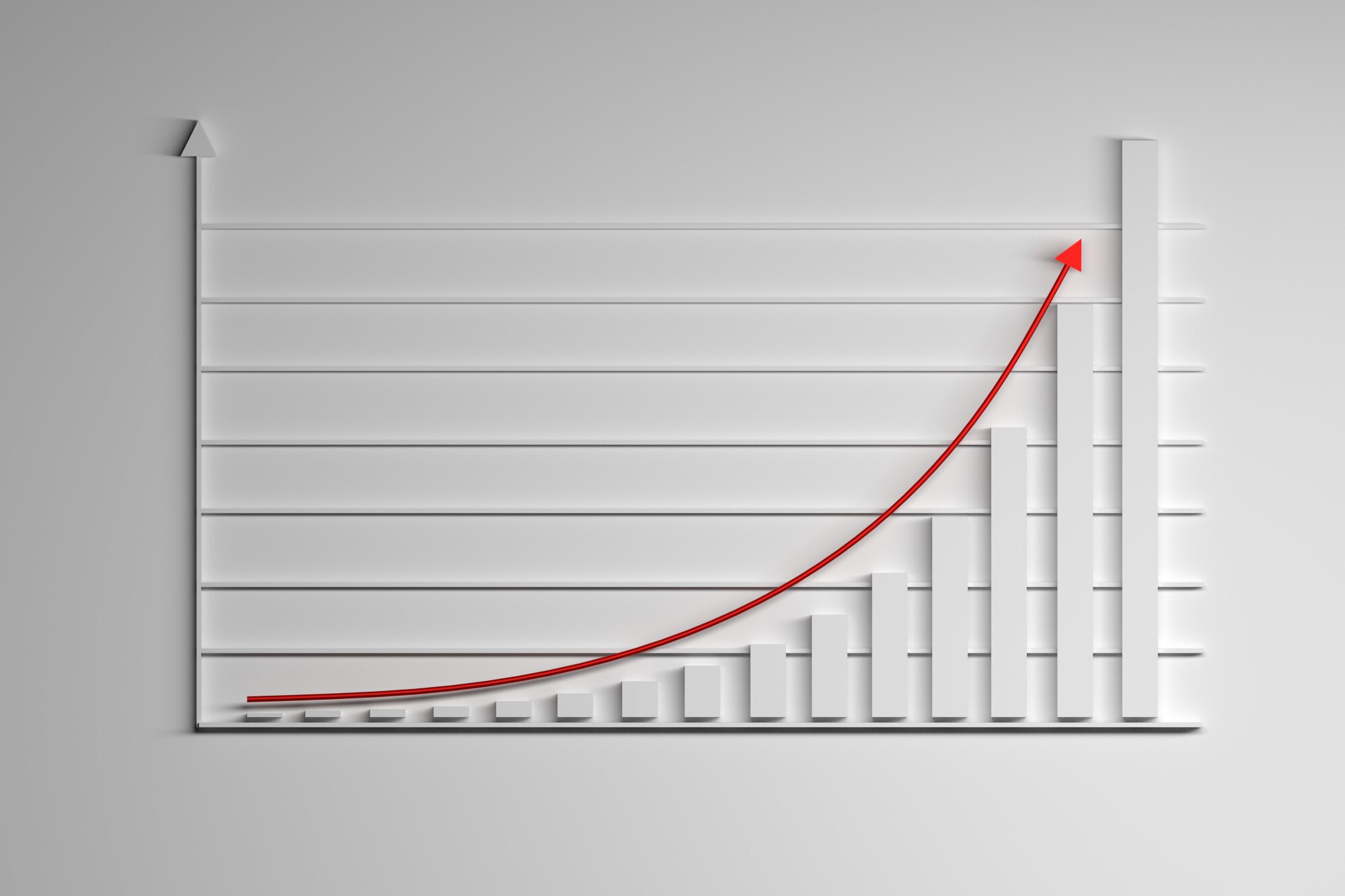
Exponential Graph: Fixed Multipliers, Curved Results

Table of Contents

An unshifted exponential graph curves because equal input steps multiply the output by a fixed factor: doubling takes 1 to 2 to 4, so the gains keep growing. A straight line adds the same amount each step instead. To sketch the curve, use a few points and the horizontal line it approaches.

Recognize Growth and Decay

In (y=ab^x), the variable sits in the exponent, with (a\ne0), (b>0), and (b\ne1). For positive (a), a base above 1 produces an increasing curve; a base between 0 and 1 produces a decreasing one.

A negative coefficient reverses that direction: where (2^x) rises from 1 to 2, (-2^x) falls from −1 to −2. Both outputs still multiply by 2. These unshifted exponential graphs follow a fixed multiplier, not a fixed increase.

Plot a Curve From Points

For an exponential graph example, use (y=2^x). Inputs (-2,-1,0,1,2) give outputs (\frac14,\frac12,1,2,4). Plot these pairs and draw a smooth curve, not straight segments.

The exponential shape gets steeper to the right and flatter to the left. Its horizontal asymptote, (y=0), guides the left tail: the outputs stay positive even as they shrink toward zero.

Choose a plotting method according to the part you need help with:

Plotting approach	Best for	Setup for y = 2^x	Pros	Cons
Hand plotting on linear graph paper	Practising coordinates	Use 1-unit ticks; x from −2 to 2, y from 0 to 4	Shows (0, 1) and increasing steepness on equal scales	Place 1/4 and 1/2 carefully near the axis
Desmos Graphing Calculator	Checking a sketch	Enter y = 2^x; x-window −4 to 4, y-window −1 to 16	Zoom and select points to inspect near y = 0	Automatic scaling can hide small positive outputs
GeoGebra Graphing Calculator	Comparing curve and asymptote	Enter y = 2^x and y = 0; x from −4 to 4, y from −1 to 16	Shows both as separate objects	Low zoom can make them appear to overlap
Spreadsheet XY scatter chart	Repeatable coordinate tables	Fill A2:A10 with −4 to 4; enter =2^A2 in B2 and fill down	Nine calculated points show successive doubling	Use markers; straight connectors mislead and smoothing only approximates

Shift, Reflect, and Scale the Curve

To move the curve without guessing, use [ y=ab^{x-h}+k. ] Each parent point ((u,v)) becomes ((u+h,av+k)): (h) shifts horizontally, (a) scales vertically and reflects when negative, and (k) shifts vertically. The asymptote moves to (y=k). Each one-unit increase in (x) multiplies the signed difference (y-k) by (b), not necessarily the output (y). The domain is all real numbers; the range is (y>k) when (a>0), and (y<k) when (a<0). Applied models may restrict the domain: for example, to nonnegative elapsed time.

For (y=2\cdot2^{x-1}-3), the function simplifies to (y=2^x-3). The asymptote is (y=-3), with range (y>-3). This exponential function graph crosses the horizontal axis because the downward shift puts some outputs below zero.

Find Intercepts With Logarithms

Finding that crossing pins down where your sketch changes sign.

The (y)-intercept comes directly from (x=0): (y=2\cdot2^{-1}-3=-2), giving ((0,-2)). For the (x)-intercept, isolate the exponential: [ 0=ab^{x-h}+k \quad\Longrightarrow\quad b^{x-h}=-\frac{k}{a}. ] The right side must be positive; zero or a negative value means no real crossing. Otherwise, [ x=h+\frac{\ln(-k/a)}{\ln b}. ] Here (2^{x-1}=3/2), placing the crossing at (x=1+\log_2(3/2)\approx1.585).

Find an Equation From Points

Working backward, points ((0,y_0)) and ((1,y_1)) determine an unshifted nonconstant exponential model when (y_0) and (y_1) are nonzero, have the same sign, and differ, through [ a=y_0,\qquad b=\frac{y_1}{y_0}. ] Thus ((0,6)) and ((1,9)) give (y=6(1.5)^x). This exponential function example separates the starting output from the multiplier.

For a known asymptote (y=k), compare distances from that line: [ a=y_0-k,\qquad b=\frac{y_1-k}{y_0-k}. ] Without the asymptote, two points generally leave a vertically shifted model undetermined.

Model Percentage Change and Continuous Growth

Suppose a population starts at 200 and grows 5% annually. The model is (y=200(1.05)^x), with (x) in years. Its exponential growth graph shows larger annual gains as the population grows. In general, a positive starting amount (A) and decimal rate (p) give (y=A(1+p)^x).

Decay uses (1-p): a hypothetical sample retaining 80% each hour follows (y=A(0.8)^x).

For continuous growth, use (y=Ae^{rx}), where (A>0) and (e\approx2.71828). The natural exponential graph is (y=e^x); positive (r) gives growth and negative (r) gives decay.

Key Takeaways

Extend a point table by multiplying outputs for an unshifted exponential, or signed differences from the asymptote for a shifted one.
Keep the asymptote separate from the horizontal axis when a curve shifts.
Match a percentage multiplier to the input’s time unit.
Use intercepts to anchor where the sketch meets the axes.

Frequently Asked Questions

How Do You Tell If a Graph Is Linear or Exponential?

Equal input steps give constant output differences for a line and constant ratios for an unshifted exponential. For a shifted exponential, compare distances from its asymptote instead.

Can an Exponential Curve Touch Its Horizontal Asymptote?

No: for these nonconstant functions, (y-k=ab^{x-h}) cannot equal zero. An apparent overlap on a screen reflects the display scale, not contact.

Why Must the Base Be Positive and Different From 1?

A positive base permits every real input, while excluding 1 prevents a constant function. A negative base fails at inputs such as (x=\frac12); gaps in such a plot are not an exponential curve’s missing tail.

Can an Exponential Function Have Negative Outputs?

Yes: a negative coefficient reflects the unshifted curve across the horizontal axis. Its range becomes (y<0), instead of (y>0) for a positive coefficient; a vertical shift can also create negative outputs.

How Can You Check Plotted Points in Desmos?

Enter the equation and a table of your inputs and calculated outputs, then compare the points with the curve. Put parentheses around the entire exponent of a transformed equation to avoid plotting a different function.

Start With Points and the Asymptote

If you need a sketch, choose hand plotting to practise placing fractional outputs; choose a calculator when you need to inspect a crossing more closely. For a model, first decide what one input step represents. An hourly retention factor cannot describe a yearly step without conversion.

Once the points are in place, give the empty space between them equal attention. In the shifted example, the crossing near 1.585 belongs between outputs of opposite signs, while the tail stays above its own limiting line. Extra points can test your drawing, but they cannot rescue the wrong shape. A faithful exponential sketch preserves the fixed multiplier in signed differences from its asymptote, including where you have plotted no points at all.