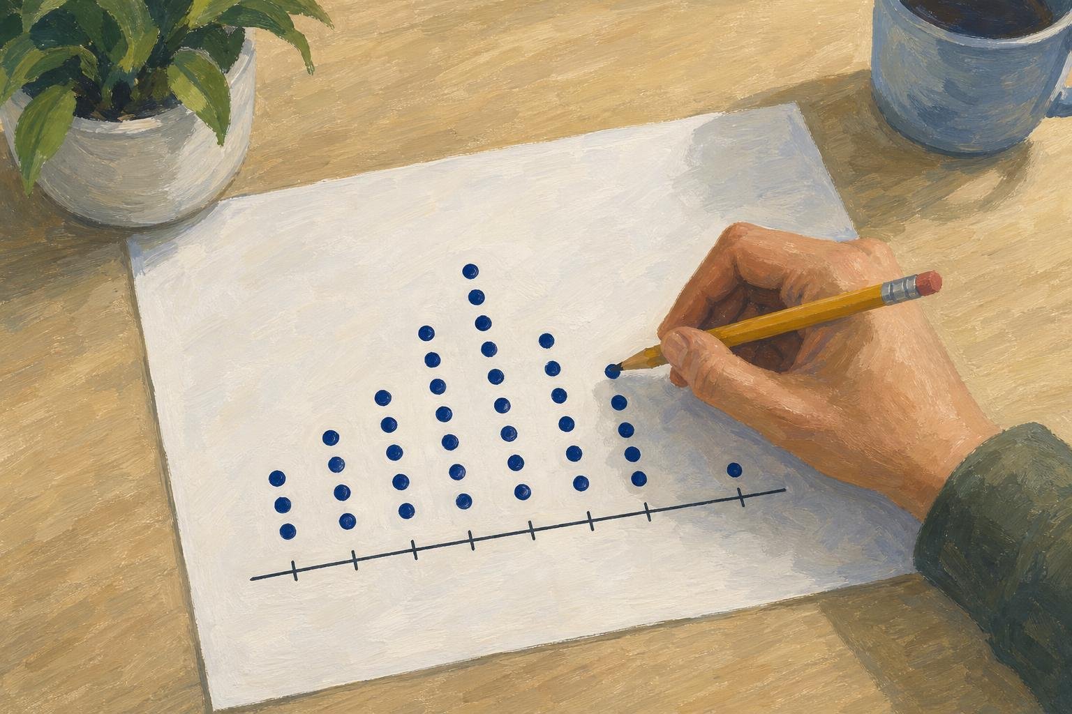
Dot Plot Explained: What Each Stacked Dot Tells You

Table of Contents

A dot plot shows numerical observations as dots above a number line, stacking repeated values so you can see each observation instead of only a bar’s total. Choose it when the individual values matter: a stack lets you count responses without hiding them inside a solid shape. The same dots can reveal a common response and a less typical one at a glance.

What Each Dot Represents

In this frequency display, one dot represents one observation. If three students report the same study time, their responses form a three-dot stack. The horizontal position answers “What value?” and the stack answers “How many?”

Those positions need a trustworthy scale. Read the title and units first, then consider this badly drawn number line:

1────2────5

It makes the difference between 1 and 2 look identical to the difference between 2 and 5. Equal spaces must mean equal numerical differences. Otherwise, even correctly counted dots tell a distorted story about how far apart the values are.

Read a Finished Example

Consider a constructed classroom dataset recording study time in hours:

1, 2, 3, 3, 4, 4, 4, 5, 5, 5, 5

The finished chart places each response above its value. Rows provide room for stacking; they do not represent separate groups of students or additional hours.

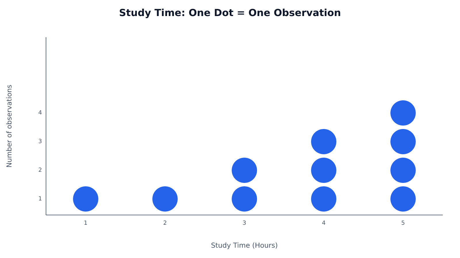
Dot plot of study time, with counts rising from one observation at 1 and 2 hours to four at 5 hours.

Count the dots in each stack, then add the counts to find the total number of observations. The responses cluster toward the higher end of the scale. Every labeled position has a response; there are no gaps across this scale.

Build Your Own Plot

To recreate that chart, sort the recorded observations so repeated entries sit together. Sorting changes their order, not their values. Cross off each entry as you plot it if that helps you avoid plotting a response twice.

Before adding dots, repair the compressed scale shown earlier. A whole-hour scale from 1 through 5 needs the intervening positions:

1────2────3────4────5

Whole-hour positions suit these observations. Measurements recorded to the nearest half hour would need positions for those halves; preserve that precision in your dot plot data.

Place a dot above each value and stack repeats with consistent spacing. Use equally sized dots so one response does not appear more important than another. Compare each stack with its entries, then count the whole chart.

Find the Center and Spread

The tallest stack gives the mode: 5 hours. With 11 observations, the median is the sixth response in the ordered list: 4 hours. The most common response and the middle response therefore differ. For an even number of observations, find the median by averaging the two middle values.

The mean uses every response. Multiply each value by its frequency and add the products: (1 × 1) + (2 × 1) + (3 × 2) + (4 × 3) + (5 × 4) = 41 hours. Divide by the 11 responses: 41 ÷ 11 ≈ 3.73 hours. Here, the mean, median, and mode are approximately 3.73, 4, and 5 hours, respectively.

The range measures spread between the endpoints: 5 − 1 = 4 hours. Yet that same range can describe either of these five-dot datasets:

A
●           ●
●     ●     ●
1  2  3  4  5

B
      ●
      ●
●     ●     ●
1  2  3  4  5

A contains 1, 1, 3, 5, 5; B contains 1, 3, 3, 3, 5. Both span four hours. A puts four responses at the endpoints, while B puts three in the middle. The range cannot distinguish them; the dots can.

Choose the Right Chart for Your Data

Use dot plots when readers need individual numerical values and can still distinguish the observations. The classroom chart makes exact counting practical. There is no universal size cutoff: repeated values build taller stacks, while closely spaced values compete for horizontal room.

For a hypothetical payroll dataset containing thousands of salaries, individual dots could bury the useful comparison. A histogram could group salaries into pay intervals, showing where employees concentrate. You would lose each person’s exact salary, but gain a readable view of the distribution. Bin boundaries affect that view, so choose intervals that serve the comparison.

The table separates that tradeoff from two other reasons to use dots: separating overlapping observations and comparing categories.

Display option	How values and frequency appear	Best for	Main advantage	Main limitation
Stacked dot plot	For values 2, 2, 3, 5: two dots at 2, one at 3, one at 5; stack height = count.	Small numerical datasets with repeated values	Preserves individual values and shows exact frequencies.	Many repeats create tall stacks; nearby values can crowd together.
Strip plot with jitter	For values 2, 2, 3, 5: four dots at their numerical positions, offset perpendicular to the value axis.	Individual numerical observations with overlapping values	Offsets separate repeated observations without changing their values on the measurement axis.	Offset height does not encode frequency; dense clusters are hard to count.
Histogram	For values 2, 2, 3, 5: bins 2–<4 and 4–<6 have counts 3 and 1 on a count axis.	Numerical distributions that become crowded as individual dots	Groups observations into intervals to reveal broader distribution patterns.	Exact values within each bin are hidden; bin boundaries affect appearance.
Category-based dot chart (Cleveland)	One dot per category shows a value, such as median rent: North $1,200; South $1,500.	Comparing numerical measures across named categories	Dot position supports direct comparisons on a shared numerical scale.	Dot count is not observation frequency; within-category distributions are hidden.

A shared numerical scale only helps when differences mean something. Apartment numbers are identifiers, not quantities: the distance between apartment 2 and apartment 5 is not a measurement of the apartments.

Recognize Other Charts That Use Dots

A Cleveland dot chart uses the category comparison shown in the table. A service desk’s average wait time, for example, would get one dot beside that desk’s name. Moving along the numerical axis means a longer or shorter wait, not more observations.

The Federal Reserve’s dot plot instead appears in its Summary of Economic Projections. It records Federal Open Market Committee participants’ assessments of appropriate monetary policy through federal funds rate projections for specified year-ends and the longer run.

Those projections can change market expectations. In the Federal Reserve’s June 16, 2021 projections, the median indicated two quarter-point rate increases by the end of 2023, compared with none in March. Reuters reported that U.S. Treasury yields rose that day as investors reacted to the shift toward earlier tightening.

The market use is forward-looking: investors compare the projected rate path with what they previously expected. The dots remain individual assessments, not an agreed schedule, and the published chart does not identify participants by name.

Key Takeaways

Keep individual dots when exact observations matter to the comparison.
Use the classroom example’s differing centers to distinguish a typical response from a calculated average.
Compare the five-dot examples before assuming equal ranges mean similar distributions.
Choose grouped intervals when individual marks obscure the pattern.
Read Fed projections as policy expectations, not recorded study-time-style observations.

Frequently Asked Questions

What Is a Dot Plot?

A dot plot marks values with dots; in a stacked frequency version, each dot represents an observation. The important distinction is whether the marks represent individual records or category summaries, as in the Cleveland chart.

What Does the Fed Dot Plot Show?

The Fed dot plot shows policymakers’ individual projections of an appropriate federal funds rate for the periods displayed. A shift in those projections signals changed assessments, not a binding commitment to future decisions.

What Does a Dot Plot Look Like?

A stacked dot plot looks like columns of dots above numerical positions, with taller columns indicating more observations. If the chart instead has named categories beside individual dots, use their positions to compare category values, not their number to count responses.

Can One Chart Have Two Equally Common Values?

Yes, exactly two values tied for the highest frequency give a dataset two modes, called bimodal. Two equally tall stacks qualify only when no other stack is taller.

Does an Empty Position on the Scale Mean the Data Is Missing?

No, an empty position usually means no recorded observation has that value. Missing data means an observation was not recorded or is unavailable; the gap alone cannot establish that.

Start With One Verified Dataset

Before sharing your first chart, check that its title identifies the observations, its axis states the unit, and equal numerical differences occupy equal spaces. Then compare each stack with the source data and confirm the total dot count. For the study-time example, the stacks should contain 1, 1, 2, 3, and 4 dots at 1 through 5 hours, respectively: 11 observations in all.