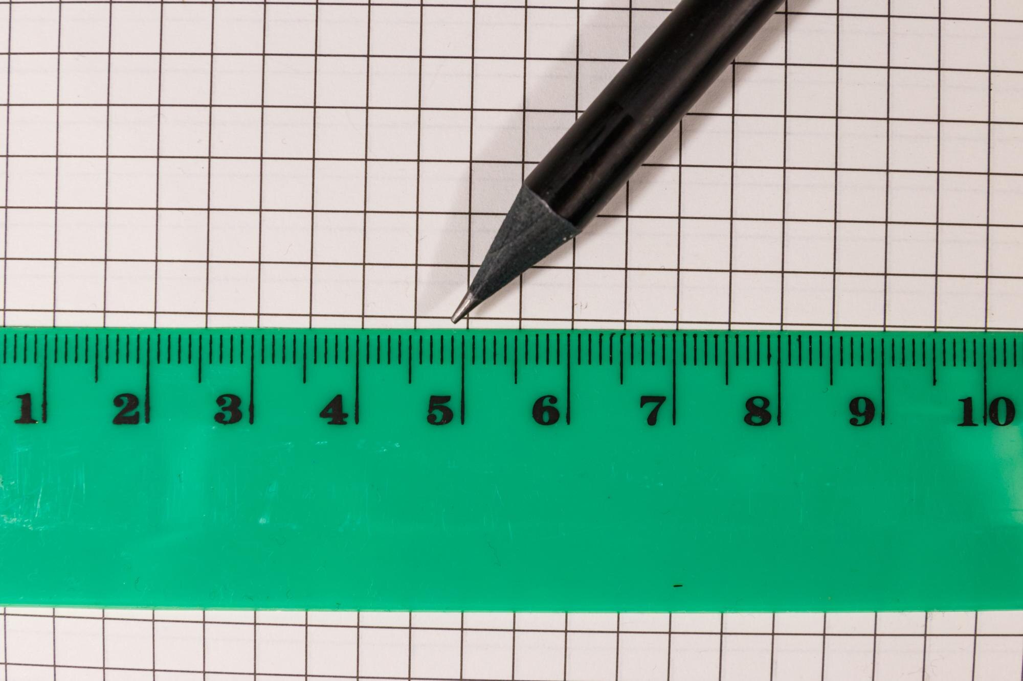
Reading a Linear Graph: Why the Slope Stays the Same

Table of Contents

A linear graph runs straight across a grid without bending or changing direction. For a nonvertical line, each equal step sideways produces the same change in height. That repeatable movement lets you turn an equation into points you can draw. A linear graph represents a linear equation as a straight line, while a line chart connects data points that may or may not lie on a straight line.

What Makes a Graph Linear?

The steepness of a nonvertical line stays constant wherever you measure it. Take two points, find the change in their y-coordinates, and divide by the change in their x-coordinates. That quotient is the slope.

In a nonvertical linear graph, the same slope carries you along the whole line. The distance between your chosen points can change; the ratio cannot. This is the defining pattern of nonvertical linear graphs:

Slope = change in y ÷ change in x

Read the Slope and Intercepts

The equation y = mx + b puts that slope beside x. Here, m is the slope and b is the y-intercept’s vertical coordinate. In y = 3x − 6, increasing x by 1 increases y by 3. The −6 places the y-intercept at (0, −6).

That point sits below the horizontal axis. To find where the line reaches the axis itself, set y to zero:

0 = 3x − 6

Add 6 to both sides, giving 6 = 3x. Divide by 3 to get x = 2. The x-intercept is therefore (2, 0): the point where the line’s height is zero.

Find an Equation From a Table

You can work backward from coordinates to an equation. Suppose a table contains (0, 3), (1, 5), and (2, 7). Each increase of 1 in x gives an increase of 2 in y, so the slope is 2. The point with x = 0 supplies the starting height, 3. Together they give y = 2x + 3.

Now suppose the next row is (4, 11). The complete table is:

x	y
0	3
1	5
2	7
4	11

The increase in y is larger, but so is the step in x. Compare the rate, not the vertical change alone:

Slope = (11 − 7)/(4 − 2) = 4/2 = 2

This matches the earlier slope, so (4, 11) also fits y = 2x + 3.

Plot a Line From Its Equation

For a linear equation graph, use the equation to choose points you can place accurately. With y = −x/2 − 2, put the first point at the y-intercept, (0, −2). The slope is −1/2: move 2 units right and 1 unit down to reach (2, −3). Another identical move reaches (4, −4).

Check that last point by substitution: −4/2 − 2 = −4. Two distinct points determine the line; the third gives you a way to catch a misplaced dot before drawing through them.

Label the axes and keep the spacing uniform along each one. For this unrestricted equation, draw a straight line through your points, adding arrowheads to show that it continues beyond the grid. Each new point follows the same movement: 2 x-units right and 1 y-unit down. Count coordinate units, not grid squares.

Use Constant Rates in Real Problems

A practical linear graph example is earnings at a fixed hourly rate. Suppose a job pays $15 per hour, with no additional payment or deductions in the model. With x for hours and y for earnings in dollars, y = 15x. After 5 hours, y = 15 × 5 = $75. Zero hours gives zero earnings, so the line passes through the origin.

That zero starting value also fits a proportional cost model. If potting soil costs $2 for 3 pounds, its unit rate is $2/3 per pound. For 6 pounds, the cost is (2/3) × 6 = $4.

A starting amount changes the equation without changing the rate. In the tank-filling example below, the 20 L already present stays separate from the water added each minute. The rate controls the change, and the starting value sets the intercept.

These models apply only to meaningful inputs. Hours, elapsed time, and soil weight cannot be negative. The filling model applies only until the tank reaches capacity; no capacity is specified here.

Constant-rate model	Rate (slope)	Variables and units	Linear equation	Worked point (x, y)	Starting value (y-intercept)
Walking at a steady speed	4 km per hour	x = time (hours); y = distance (km)	y = 4x	At 3 hours: y = 4 × 3 = 12 km; (3, 12)	0 km
Filling a tank containing 20 L	6 L per minute	x = filling time (minutes); y = water volume (L)	y = 6x + 20	At 5 minutes: y = 6 × 5 + 20 = 50 L; (5, 50)	20 L
Printing with a setup fee	$0.10 per page	x = pages printed (0, 1, 2, …); y = total cost ($)	y = 0.10x + 3	At 40 pages: y = 0.10 × 40 + 3 = $7; (40, 7)	$3 setup fee
Draining a tank containing 100 L	−5 L per minute	x = draining time (minutes), 0 ≤ x ≤ 20; y = water volume (L)	y = 100 − 5x	At 8 minutes: y = 100 − 5 × 8 = 60 L; (8, 60)	100 L

For the draining model, draw only the segment from (0, 100) to (20, 0): the tank is empty after 20 minutes. For printing, plot separate points at whole-number page counts; do not connect them as though fractional pages were possible.

Handle Horizontal and Vertical Lines

The draining tank has a changing height; a horizontal line such as y = 4 does not. Its y-value stays fixed while x varies, giving a slope of zero. It still defines y as a function of x.

Turn the line vertically and the roles change. For x = −3, x stays fixed while y can vary, so the line cannot assign just one output to that input. It is the graph of a linear equation, but y = mx + b cannot describe it: every slope calculation would divide by zero.

Key Takeaways

When reading an equation, separate the starting value from the amount of change.
When comparing table rows, account for the horizontal step as well as the vertical one.
When plotting, use an extra point to catch mistakes before drawing.
When modeling a quantity, keep its units attached to the calculation.

Frequently Asked Questions

The equation 2x + 4y = −8 connects the first three answers: it gives one concrete line to identify, test, and plot.

What Is a Linear Graph?

A linear graph is a straight line representing the solutions of a linear equation in two variables. For example, each point on the graph of 2x + 4y = −8 supplies an ordered pair that makes that equation true.

Is Every Linear Relationship Proportional?

No. A proportional relationship has the form y = kx, and its graph passes through the origin. For the equation above, rearranging gives y = −x/2 − 2. Its nonzero y-intercept, −2, means the relationship is linear but not proportional.

How Do You Graph 2x + 4y = −8?

Plot its intercepts, (0, −2) and (−4, 0), and draw a straight line through them. Alternatively, rearrange it as 4y = −2x − 8, then y = −x/2 − 2, and use the slope movement demonstrated earlier.

What Are the 7 Rules of Graphing?

A seven-step routine can organize your work. Identify the variables; label the axes; choose uniform scales; find an intercept or starting point; calculate another point; draw the appropriate line; and test an additional point.

Is y = −2x + 3 a Linear Equation?

Yes, y = −2x + 3 is linear because it has the form y = mx + b. Its slope is −2 and its y-intercept is 3, so it falls 2 units for every 1-unit move right.

Can a Vertical Line Represent a Linear Equation Without Representing a Function of x?

Yes: x = 5 is a linear equation whose vertical graph does not represent a function of x. The input 5 corresponds to more than one output, which prevents it from being a function.

Turn an Equation Into a Line

Try a fresh equation: 3x + 2y = 12. Find both intercepts, draw the line, and test whether (2, 3) lies on it before reading the answer.

Setting x = 0 gives y = 6, so the y-intercept is (0, 6). Setting y = 0 gives x = 4, so the x-intercept is (4, 0). Draw the line through those points. To check (2, 3), substitute: 3 × 2 + 2 × 3 = 12. The equation holds, so the point lies on the line.