
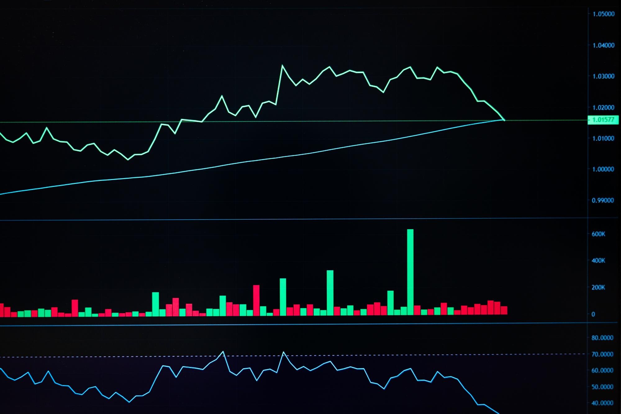

A spaghetti plot overlays individual lines on shared axes, forming a tangle wherever their paths cross or bunch together. Each line follows one subject, group, or forecast run, so you can see differences that an average would hide. Three subjects with opposing paths make that contrast easy to see.
In This Article
- Read the Axes Before Following a Line
- Build a Small Example Without Joining Different Subjects
- Separate the Average From Individual Variation
- Reduce Clutter Without Hiding the Comparison
- Split the View When Overlap Blocks Reading
- Understand What Weather Forecast Lines Represent
- Key Takeaways
- Frequently Asked Questions
- Choose the View That Preserves Comparison
Read the Axes Before Following a Line
Read the chart in this order: identify the units, follow individual paths, then compare them with the summary. In a repeated-measures chart, each line connects observations from the same subject. The horizontal axis might show weeks since treatment; the vertical axis might show a measured score.
Those axes give a slope its meaning: a rise over one week represents faster change than the same rise over two weeks. Follow the recorded points to see where a subject changes direction. In the example below, two subjects reach the same score at week 1, then head in opposite directions.
Build a Small Example Without Joining Different Subjects
Consider these invented scores for three subjects measured at weeks 0, 1, and 2:
| Subject | Week 0 | Week 1 | Week 2 |
|---|---|---|---|
| A | 2 | 4 | 6 |
| B | 6 | 4 | 2 |
| C | 3 | 3 | 3 |
A rises, B falls, and C stays level. The X marks the intersection of A and B at week 1.
Score
  6 | B               A
    |   \           /
  5 |     \       /
    |       \   /
  4 |         X
    |       /   \
  3 | C---/---C---\---C
    |   /           \
  2 | A               B
    +------------------
      0       1       2
              Week
This Python code reproduces the plot and adds a dashed mean. It requires pandas and Matplotlib.
import pandas as pd
import matplotlib.pyplot as plt

wide = pd.DataFrame({
    "subject": ["A", "B", "C"],
    0: [2, 6, 3],
    1: [4, 4, 3],
    2: [6, 2, 3],
})
df = wide.melt(
    id_vars="subject",
    var_name="week",
    value_name="score"
)
df["week"] = df["week"].astype(int)

fig, ax = plt.subplots(figsize=(6, 4))
for subject, rows in df.groupby("subject"):
    rows = rows.sort_values("week")
    ax.plot(
        rows["week"], rows["score"],
        marker="o", label=f"Subject {subject}"
    )

mean = df.groupby("week")["score"].mean()
ax.plot(
    mean.index, mean.values,
    color="black", linestyle="--",
    linewidth=3, label="Mean"
)
ax.set(
    xlabel="Week", ylabel="Score",
    xticks=[0, 1, 2], ylim=(1.5, 6.5)
)
ax.legend()
fig.tight_layout()
plt.show()
The long table has one row per subject-week observation. Grouping by subject and sorting by week keeps each path intact; plotting the whole table as one series would connect different people.
In Microsoft Excel, put week in the first column and give each subject a separate series. An XY scatter chart with straight lines and markers preserves numeric time spacing, including unequal intervals.
Separate the Average From Individual Variation
The code draws the mean as a thick, dashed black line so it stands apart from the subjects. A median is another option when the middle observation answers your question better; label the summary you choose. With missing visits, changing membership can also move that summary.
A standard-deviation band describes the spread of subjects, while a confidence interval describes precision of the estimated average: even a narrow interval can sit among widely scattered paths. Calculating that precision for repeated measurements requires accounting for dependence within subjects.
Here, the mean stays the same at every week. Whether a higher score means improvement depends on the measure, but the numerical result is clear: the flat mean hides A’s rise and B’s equally large fall.
Reduce Clutter Without Hiding the Comparison
Highlight A in a strong color and draw the other subjects as thin gray lines. An endpoint label lets readers find A without repeatedly consulting a legend, while B remains visible as its opposing trajectory.
Transparency helps with overlap, but consider an imagined chart of 100 patients whose scores remain identical through week 1. Their transparent segments pile onto the same path; the dark stroke hides how many patients it contains. Darkness cannot reliably establish a subject count.
Markers make the actual visits visible. If A missed week 1, show that absence explicitly, for example by breaking the line there; a connecting segment alone supplies no measurement at the missing visit.
Split the View When Overlap Blocks Reading
Small multiples give each subject or group a separate panel. Shared horizontal limits and a common vertical scale support direct comparisons of magnitude and slope. With independent vertical scales, small fluctuations in C in another dataset could fill a panel as dramatically as A’s larger change.
For additive quantities, a stacked area chart can show how components contribute to a total. The subjects’ scores here call for comparing paths, so keep their baselines aligned.
Repeated-background panels preserve that alignment while reducing competition for attention. Give A its own panel with B and C subdued behind it, then repeat for the other subjects. Each path gets a clear foreground without losing its comparison group.
Understand What Weather Forecast Lines Represent
Weather spaghetti charts often compare ensemble forecasts produced with different initial conditions or model configurations. NOAA’s Global Ensemble Forecast System, or GEFS, is one such system: its members can produce different tracks for the same hurricane. Those lines represent modeled futures, unlike the observed subjects in the table.
If the hurricane tracks diverge, the forecast offers a wider range of possible routes. That spread helps explain why one modeled track cannot stand for the whole ensemble; the outermost tracks do not automatically enclose a calibrated probability or confidence interval.
Other weather spaghetti plots overlay forecast contours, such as a specified atmospheric-height contour. Their crossings compare the forecast positions of that contour, not storm routes. Even closely clustered forecasts can share an error.
Key Takeaways
- Define the unit behind a line before interpreting its shape.
- Keep opposing trajectories visible when presenting an average.
- Use a highlighted foreground for a focused comparison.
- Give every subject a panel when every path needs inspection.
- Use stacked areas for additive composition, not as a substitute for separating subjects.
Frequently Asked Questions
How Do You Read a Spaghetti Plot?
Trace a labeled line through its recorded points, using both axes to interpret change. At a crossing, follow its color or markers onward instead of switching to the intersecting path.
What Is the Difference Between a Spaghetti Plot and a Line Plot?
A spaghetti plot is a multi-series line plot emphasizing individual trajectories on shared axes. Build it by assigning a separate series to each subject; it needs no special chart type.
What Is a Spaghetti Chart Used For?
It shows how trajectories differ across subjects or forecast runs. For repeated patient measurements, it can reveal who reverses direction even when the group summary stays steady.
Should Small-Multiple Panels Share the Same Vertical Scale?
Yes, when readers need to compare absolute values or slopes directly. Independent scales suit inspecting within-panel patterns, provided each panel’s scale is clearly labeled.
Can I Highlight One Group While Keeping Every Other Group Visible?
Yes: style the selected group distinctly and leave all other lines visible in subdued gray. Draw the background lines first so the selected path remains on top at crossings.
Choose the View That Preserves Comparison
At weeks 0 and 2, this dataset contains exactly the same scores: 2, 3, and 6. Unlabeled endpoint snapshots would look unchanged, even though A and B have exchanged positions. Retaining subject identity changes the question from whether the group’s distribution changed to whose score changed, and in which direction.
That distinction is the example’s central result: stability in the distribution does not imply stability for the people represented. The connecting paths make that difference visible, rather than leaving readers to infer individual changes from a group summary.
Recommended for you

Comparing Histogram vs Bar Graph: What Values Reveal
The histogram vs bar graph choice starts with categories versus numerical observations. Learn how bins and axes shape each chart, and see which fits your data.
Velocity vs Time Graph: Slope, Area and Reversed Motion
Read a velocity vs time graph using a runner and a reversing cart. Connect slope to acceleration and signed area to displacement. See how motion adds up.

Bode Plot Gain and Phase: Where Feedback Can Go Wrong
Read a bode plot's gain and phase together to avoid misleading stability judgments. Learn where to measure gain and phase margins; see the worked example.

Behind an Absolute Value Graph: The Sharp Corner Explained
An absolute value graph has two rays and a sharp vertex. Learn how the equation sets its shape, range, and intercepts, then plot it correctly. See how here.
Dot Plot Explained: What Each Stacked Dot Tells You
A dot plot puts each observation above a number line. Learn how stacked dots show frequency and why equal spacing matters. See the study-time example.
Explained: How to Read a Histogram, From Axes to Area
Learn how to read a histogram using book-length examples. Check axes, interpret counts, and see why unequal bin widths need area. Read the walkthrough.
Pie Chart Examples: The Dollar Totals Behind Each Slice
Use pie chart examples with a $4,000 budget and $100,000 in sales to connect slices to dollars, calculate shares, and compare totals. See the calculations.

Venn Diagram: Why Club Rosters Can Count Students Twice
A Venn diagram explains how 18 art-club and 14 music-club members fit in a class of 30. Learn to read overlaps and avoid double counting. See how it works.