
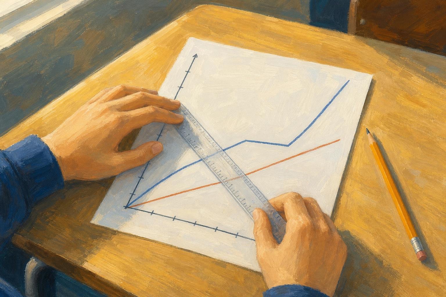

A distance time graph shows how distance changes as time passes. When distance means total distance traveled, its slope gives speed, not its height. For distance from a starting point, the slope’s magnitude gives speed only when motion is directly toward or away from that point. Suppose a truck’s graph reaches 16 miles and someone calls that 16 miles per hour: they have read a distance as a speed. The missing information is how long the truck took to cover that distance.
The examples below turn that mistake into a way to read stops, changing speeds and whole journeys. One distinction governs them all: does “distance” mean total travel or distance from a starting point?
In This Article
- Read the Labels and Scales
- Understand Straight and Horizontal Segments
- Calculate Speed Between Two Points
- Find the Average for the Whole Journey
- Estimate Speed on a Curved Line
- Compare Two Travelers on One Graph
- Distinguish Distance Plots From Speed Plots
- Key Takeaways
- Frequently Asked Questions
- Read the Axes Before Calculating
Read the Labels and Scales
Suppose a bus leaves York station, with its journey recorded on a graph. Time normally runs along the horizontal axis and distance along the vertical axis. If the label says “distance from York station,” a return toward the station will lower the line; “total distance traveled” records something different.
That bus journey also gives the grid a meaning. If four equal divisions cover an hour, each represents 15 minutes. One square need not equal one unit, and the axes need not use matching scales. If recording begins after departure, the bus may already be some distance from the station. Its starting height tells you where it is, not how fast it is moving.
Understand Straight and Horizontal Segments
On a distance time graph, constant speed appears as a straight, rising segment when the vertical axis measures accumulated travel. The bus covers equal distances in equal times. On the same cumulative-distance graph with uniform linear scales, a steeper segment means greater speed; the distance and time axes need not use matching scales. When comparing visual steepness across separate graphs, however, the corresponding axes must use the same scales.
Now give the bus a 30-minute stop. Its line runs horizontally because the plotted distance does not change. In the usual model of travel along a route, that flat section means the bus is stationary.
Exception: distance from a point: Moving in a circle centered on the station keeps that distance constant, so a horizontal line need not mean a stop. Returning directly toward the station would produce a falling line on that distance-from-station graph, but never on a total-distance graph: the return still adds travel.
Calculate Speed Between Two Points
Return to the truck from the opening. In this imagined journey, its cumulative distance rises from 4 miles at 1 hour to 16 miles at 1.5 hours. To find its average speed over that interval, subtract the two distance readings and the two time readings:
Average speed = change in cumulative distance ÷ elapsed time
The truck covers 12 miles in 0.5 hours, giving an average speed of 24 miles per hour. Dividing 16 by 1.5 would include earlier travel instead of isolating this stretch. The endpoint cannot tell the whole story.
For a straight segment, choose widely separated, clearly readable points to reduce the effect of reading errors. Keep both points on that segment. On a falling distance-from-home segment along a direct route, the gradient is negative; speed is its positive magnitude.
Find the Average for the Whole Journey
Averaging the moving speeds can give the wrong journey average: it gives unequal-duration intervals equal weight and ignores stops. A cyclist’s rest belongs in the clock time even though it adds nothing to the mileage.
Suppose the cyclist covers 6 miles in half an hour, rests for half an hour, then covers another 6 miles in one hour. That is 12 miles in 2 hours, so the whole-journey average is 6 miles per hour.
Average speed = total distance traveled ÷ total elapsed time
On a cumulative distance graph, subtract the first reading from the last to find travel during the displayed interval. On a distance-from-home graph with a return trip, add the outward and return lengths instead. Arriving home does not erase the miles ridden.
Estimate Speed on a Curved Line
A car braking gives a curve a physical meaning. On a cumulative-distance plot, the line keeps rising while the car moves, but becomes flatter as its speed falls. A curve growing steeper would show increasing speed.
Joining two points on that curve with a straight line creates a chord. Its gradient gives the average speed between those times, so it cannot isolate the car’s speed at one moment during braking.
For that moment, draw a tangent following the curve’s local direction. Calculate Δdistance ÷ Δtime using two convenient points on the tangent; they need not lie on the curve. If it rises 3 miles across 0.1 hours, the estimated instantaneous speed is 30 miles per hour. Drawing and reading introduce uncertainty, so report only the precision the graph supports.
Compare Two Travelers on One Graph
In an imagined race from York station toward a riverside finish gate, Maya starts 2 miles ahead of Leo on the same road. Leo’s line rises more steeply. Their intersection marks his catch-up point because both lines record position along that road from the same reference point.
The starting coordinates matter too: a line beginning later can indicate delayed departure, while a higher starting point can indicate a head start. The label determines whether that height represents prior accumulated travel or a position farther along the route.
An intersection alone establishes equal plotted distance at the same time. Travelers on different roads could be equally far from home without meeting. After the crossing in Maya and Leo’s race, compare line heights to see who is farther along.
Distinguish Distance Plots From Speed Plots
The race’s rising lines cannot be interpreted the same way if the vertical label changes to speed. On speed–time graphs, height gives speed directly, slope gives the rate of change of speed, and area gives distance traveled. Speed cannot be negative. For the straight-line examples below, take the direction of travel as positive; the speed–time slope then also gives acceleration. A speed graph alone cannot reveal acceleration caused by changing direction.
The table shows why identical-looking segments on distance time graphs and speed–time graphs can describe different motion.
Distance–time graph vs speed–time graph: four worked examples
| Graph and segment | Motion identified | Gradient meaning | Distance travelled in 5 s | Common reading error |
|---|---|---|---|---|
| Distance–time: rises linearly from 0 m to 20 m in 5 s | Constant speed of 4 m/s | Speed = 20 ÷ 5 = 4 m/s | Change in distance = 20 − 0 = 20 m | Treating the 20 m height as speed |
| Distance–time: stays at 20 m for 5 s | Stationary for 5 s | Speed = 0 ÷ 5 = 0 m/s | Change in distance = 20 − 20 = 0 m | Assuming a height of 20 m means continued movement |
| Speed–time: stays at 4 m/s for 5 s | Constant speed of 4 m/s | Acceleration = 0 m/s² | Rectangle area = 4 × 5 = 20 m | Treating zero gradient as zero speed |
| Speed–time: rises linearly from rest | Uniform acceleration from rest | Constant acceleration | Triangle area | Using final speed × time |
Key Takeaways
- Use the axis labels to decide which calculation applies.
- Interpret a horizontal distance segment as a stop only when the route model supports it.
- Match the distance change to the elapsed time for your chosen interval.
- Include rests when calculating a whole-journey average.
- Keep total travel separate from distance from the starting point.
Frequently Asked Questions
These questions address choices that can change an otherwise correct calculation.
What Are the Three Types of Distance-Time Graph?
The three commonly taught patterns are a rising straight line, a horizontal line and a curve. They represent constant speed, rest and changing speed in the standard cumulative-distance model, though journeys can combine them. Classify each segment separately.
How Can I Calculate the Average Speed From a Distance-Time Graph?
Use average speed = total distance / total elapsed time, including stops in the elapsed time. On a cumulative-distance graph, subtract the first distance reading from the last for the chosen interval. A final distance-from-home reading can omit return travel. Add every traveled portion before dividing.
Can a Line Slope Downward If the Graph Shows Total Distance Traveled?
No, total distance traveled cannot decrease. A downward segment indicates a labeling or plotting error, not a subtraction of return mileage. Keep adding distance during the return.
Why Must Minutes Be Converted to Hours When Calculating km/h?
Kilometers per hour requires time expressed in hours. Divide minutes by 60 before calculating, or convert a distance-per-minute result afterward. Match the denominator to the requested unit.
Can Two Journeys Be Compared If Their Graph Scales Differ?
Yes, compare coordinate values and calculated speeds instead of visual steepness. A compressed time axis can make the same journey look steeper. Replot on common axes to compare timing and progress visually.
Read the Axes Before Calculating
Before calculating, check the axis labels and scales, then choose the interval or instant the question asks about. State any route assumption your interpretation needs. Keep intermediate calculations unrounded where possible, and give the final answer its units and only the precision the graph supports.
Recommended for you

What Is a Diagram? Explanation, Not Just Illustration
What is a diagram? Learn how labeled shapes and connecting lines explain relationships, how diagrams differ from drawings, and how to read one. Read on.
Symmetric Histogram: Balance Beyond the Tallest Bar
A symmetric histogram mirrors bars around a center, not always its tallest peak. Compare tails and see how bin boundaries affect balance. Read the example.

Histogram Patterns: What Clinic Waiting Times Reveal
A histogram turns clinic waiting times into visible clusters and gaps. Learn what bins and bar heights mean, and how to choose bin widths. See the example.

SEO Infographic: Why the Publishing Page Matters Too
An SEO infographic needs more than an image. Connect your search question, visual, file and publishing page in five steps to make it useful. See the steps.

Turning Data into Stories: The Psychology of Visual Complexity
A network map with 1,200 nodes feels mesmerizing until your eyes start to swim; a five-bar chart can feel banal yet instantly graspable. The gap between awe and overload is not just taste—it’s how our visual and cognitive systems negotiate complexity, novelty, and control. If you want to use complex visuals to create connection and […]

How to Make an Infographic: A Worked Canva Example
Learn how to make an infographic in Canva, from a clear brief to a readable design, using a fictional maintenance log. Follow the step-by-step walkthrough.

A Circle Graph’s Largest Slice Isn’t Always a Majority
Read a circle graph without mistaking the largest slice for a majority. Follow a 40-student survey from counts to percentages and angles. See how it works.

Tree Diagram Rules: Clear Branches, No Loops Allowed
Learn how a tree diagram connects roots, children and leaves, then follow paths and calculate probabilities without confusing it with a flowchart. Read more.