
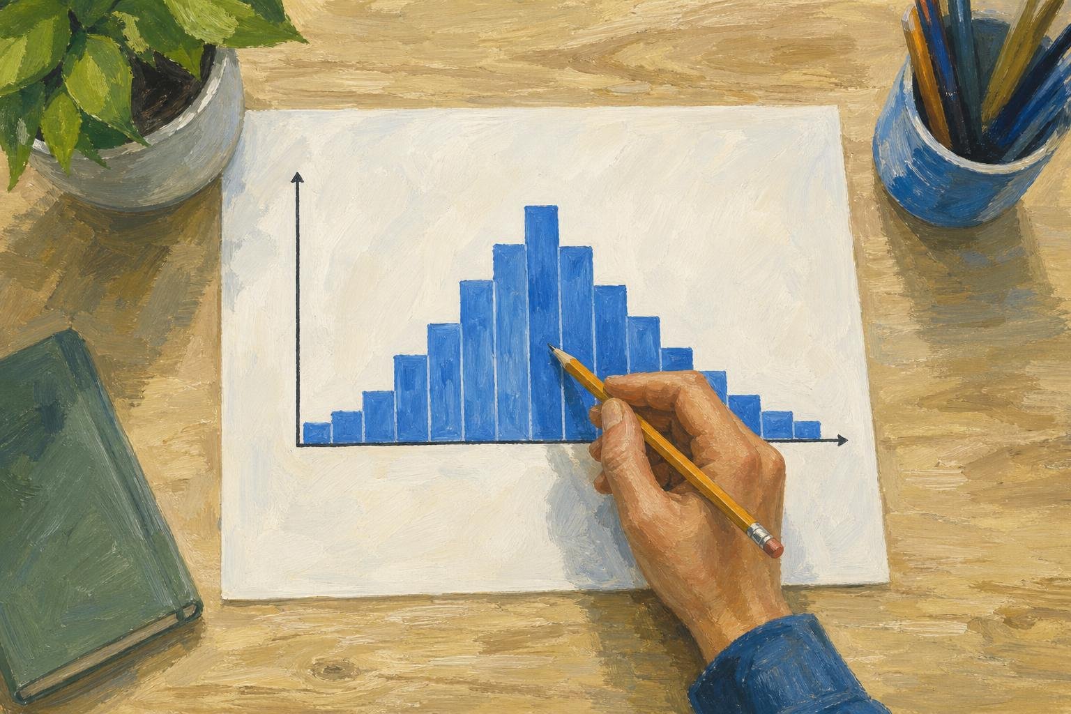

In a symmetric histogram, bars on opposite sides of the center look roughly like mirror images. Check that balance across the whole display, tails included. Using the practice scores below, you can locate the center and see how shifting bin boundaries changes your assessment.
In This Article
- What Does a Balanced Shape Look Like?
- Read a Small Example
- Separate Symmetry From Other Shapes
- Compare the Tails, Not Just the Peaks
- See How the Bins Change the Picture
- Understand What the Center Tells You
- Key Takeaways
- Frequently Asked Questions
- What the Practice Scores Show
What Does a Balanced Shape Look Like?
Imagine folding the histogram down the middle: bars at equal distances on either side should be similar in height. Compare pairs from the center outward, checking even the sparsely occupied ends. This gives you a consistent test for judging the shape of histograms.
That fold does not have to cross the tallest bar. When two matching peaks appear, the valley between them marks the center.
Read a Small Example
Suppose you group hypothetical practice scores into five intervals of equal width. Include each interval’s lower endpoint, but leave out its upper endpoint.
| Score Interval | Number of Scores |
|---|---|
| 0 to under 10 | 2 |
| 10 to under 20 | 4 |
| 20 to under 30 | 8 |
| 30 to under 40 | 4 |
| 40 to under 50 | 2 |
Around 25, the outer bars match exactly, and so do the next two bars inward. The middle interval crosses the fold, so it needs no partner.
But the same table could come from these raw scores:
0, 1; 10, 11, 12, 13; 20, 21, 22, 23, 24, 25, 26, 27; 30, 31, 32, 33; 40, 41.
The raw values, however, are not symmetric around 25. To mirror 0 across that center, you would need 50, which is missing. Only the grouped counts are symmetric; the table hides where individual scores fall within each bar.
Separate Symmetry From Other Shapes
Although the table shows one peak, symmetric histograms can have two peaks or be flat. In a roughly uniform histogram, bars have similar heights throughout the range. Both labels can describe the same shape of distribution: “uniform” refers to occupancy, while “symmetric” refers to balance.
For a physical example with two peaks, consider a pendulum. It slows near either turning point but passes quickly through the middle. If you record its position at equal time intervals during steady, symmetric oscillation, readings collect more often near the two ends.
Despite its balance, that two-peak pattern is not normal. A normal distribution follows a specific bell shape that tapers smoothly away from the center. Symmetry alone cannot establish normality. Even a roughly bell-shaped sample does not prove an exact normal model.
Compare the Tails, Not Just the Peaks
Look beyond the central peak: the edges may reveal an imbalance that the middle hides. A longer right tail suggests right skew, while a longer left tail suggests left skew. The tail determines the direction, not the tallest bar. Compare both the number of observations at each end and how far they extend.
If you spot an isolated reading at either end, give it attention rather than dismissing it. Check what it represents before calling it an error.
See How the Bins Change the Picture
Simply moving the bin boundaries can change how balanced the practice scores appear. The table compares two groupings of the same observations, each with intervals 10 points wide. In the second, boundaries fall at values ending in 5 rather than multiples of 10.
| Original Interval | Count | Shifted Interval | Count |
|---|---|---|---|
| 0 to under 10 | 2 | −5 to under 5 | 2 |
| 10 to under 20 | 4 | 5 to under 15 | 4 |
| 20 to under 30 | 8 | 15 to under 25 | 5 |
| 30 to under 40 | 4 | 25 to under 35 | 7 |
| 40 to under 50 | 2 | 35 to under 45 | 2 |
Matching bars flank the central peak in the original grouping. Shift the boundaries, and the two middle intervals instead contain 5 and 7 scores. Some scores from the original middle group now occupy a bin alongside scores in the thirties.
Bin width also affects the picture: wider bins hide differences by combining them. Narrower bins reveal more detail, but a small sample may then look jagged. Try another reasonable width and boundary position before deciding that the apparent balance holds up.
Understand What the Center Tells You
The middle observation can stay unchanged even as a large value in the right tail pulls the mean rightward.
With exact symmetry in a finite dataset, the mean and a median share the center. Visual balance alone only suggests closeness. A symmetric distribution also has its mean at the center, provided that mean is finite. Neither case depends on having a single central mode.
That central balance says nothing about spread: symmetric data may cluster tightly or stretch widely. Describe this separate feature with a spread measure, such as standard deviation or interquartile range.
Key Takeaways
- Judge symmetry by the balance of the whole display, tails included.
- Neither the number of peaks nor normality determines whether a display is symmetric.
- Check raw values for positions within bins that grouping hides.
- Changing bin widths or moving boundaries can change how symmetric a histogram looks.
Frequently Asked Questions
How to tell if a histogram is uniform, symmetric, or skewed?
Look for similar bar heights to identify uniformity, mirrored sides for symmetry, and a longer tail for skewness. Judge each feature separately: a flat histogram with balanced sides is both uniform and symmetric.
Can you give me an example of a symmetric histogram?
Look at the practice-score table above for an example centered on 25. The matching outer pairs make its bins exactly symmetric.
Must every pair of bars match exactly for a sample to look symmetric?
No, opposing bars can differ slightly without spoiling the sample’s overall balance. Even with a symmetric population, random sampling can produce small mismatches in bar heights.
Can a symmetric histogram have more than one peak?
Yes, peaks on either side of the center can mirror each other. Several peaks may point to separate groups, but the histogram alone cannot explain why they occur.
Do symmetric distributions always have a mean?
No. The Cauchy distribution is symmetric, but its population mean and variance are both undefined. You can still calculate an arithmetic mean for a finite sample of ordinary real-valued observations. That sample calculation does not establish a population property.
What the Practice Scores Show
For these practice scores, bins starting at 0 with a width of 10 give counts that are exactly symmetric around 25. Moving the boundaries by 5 breaks that exact symmetry. The claim concerns the histogram, not whether the raw scores themselves mirror around 25.
“Approximately symmetric” allows for small differences within a pattern that is balanced overall. If reasonable regrouping changes that assessment, qualify the label by noting the bin choices and visible imbalance. Keep center and spread separate: the center locates the observations, while a spread measure shows how widely they are scattered.
Recommended for you
Box Plot Reading: A Shorter Box Doesn’t Mean Faster
A box plot shows center and spread, not speed alone. Use task-time examples to compare medians and variability on the same scale. See the worked example.
Venn Diagram: Why Club Rosters Can Count Students Twice
A Venn diagram explains how 18 art-club and 14 music-club members fit in a class of 30. Learn to read overlaps and avoid double counting. See how it works.

Histogram Patterns: What Clinic Waiting Times Reveal
A histogram turns clinic waiting times into visible clusters and gaps. Learn what bins and bar heights mean, and how to choose bin widths. See the example.
Bubble Chart Accuracy: Why Area Matters More Than Radius
A bubble chart can turn a fourfold rise into a sixteenfold area. Learn to read axes and size, avoid misleading circles, and choose a design. See the guide.

Climate Change Infographic: From Emissions to Action
See how a climate change infographic links heat-trapping gases to rising heat, then separates emissions cuts from adaptation. Explore the causes and actions.
Bar Graph Scales: How Small Changes Look Much Bigger
A bar graph can make 35% to 39.6% look like a huge leap. Learn how scales and layouts shape comparisons, then build one from a small table. See the guide.
Line Graph Scales: Why the Same Data Can Look Different
A line graph can exaggerate a modest change. Learn to check axes, read a five-month sales example and build clearer charts from your data. Explore the article.
Frequency Histogram: Every Bar Traced to Its Scores
A frequency histogram shows how common scores are, not how high. Check interval boundaries, trace bars to scores, and avoid misreading the chart. See how.