
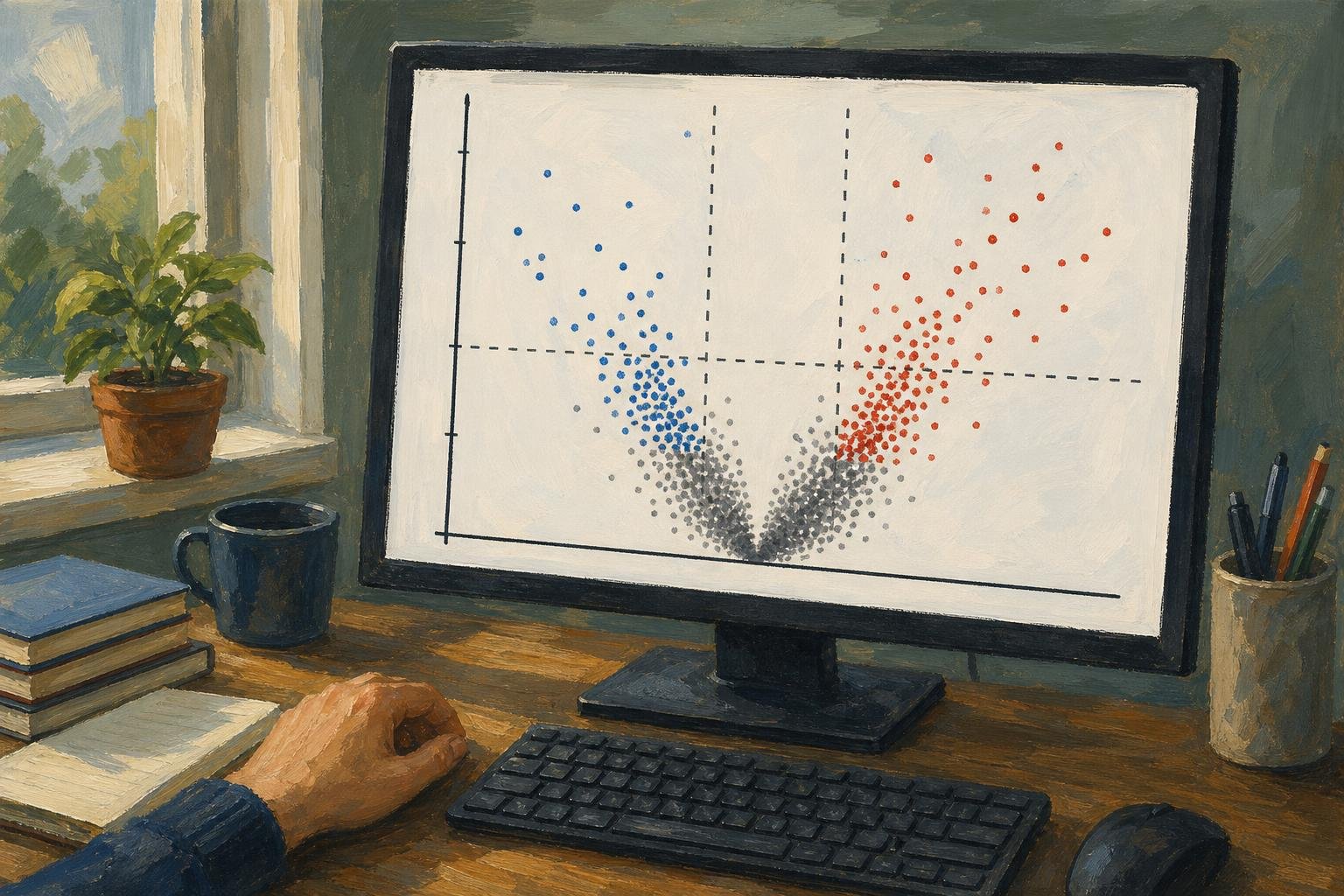

A volcano plot shows estimated change between two groups on the horizontal axis and statistical significance on the vertical axis. Chasing only its highest dots can send you after tiny effects while overlooking larger changes with less certain estimates. Each dot usually represents a gene, protein, or metabolite; the useful reading is a sequence: establish direction, read both coordinates, then decide what qualifies for follow-up.
In This Article
- Read the Two Axes Together
- Establish Which Group Is the Reference
- Understand What the Cutoffs Select
- Walk Through an Annotated Example
- Make the Plot in R
- Check the Analysis Before Choosing Hits
- Choose Another Display When It Answers More
- Key Takeaways
- Frequently Asked Questions
- Start With a Clearly Defined Comparison
Read the Two Axes Together
The tallest point is not necessarily your strongest biological candidate. Height usually represents −log10 of a p-value or adjusted p-value: smaller probabilities put dots higher. A precisely estimated, small change can therefore tower over a large, uncertain one.
That small change sits near zero on the horizontal axis, which usually shows log2 fold change. Zero means no estimated difference; positive values indicate higher abundance in the numerator group, and negative values indicate lower abundance. Moving one unit changes the abundance ratio by a factor of two.
Read across before reading up. Distance from zero tells you the estimated magnitude; height tells you the statistical evidence attached to it. The vertical-axis label determines whether that evidence uses raw probabilities or values adjusted for multiple testing. Those are different selection rules, even when the figures look alike.
Establish Which Group Is the Reference
A reversed contrast can reverse the biological story. Suppose a hypothetical paper describes a target gene as increased after treatment, but its analysis actually divides control by treatment. Its positive fold change supports higher abundance in control. Calling that treatment induction would turn the result backward, even if every plotted coordinate were calculated correctly.
The contrast, not the color, settles the direction. In DESeq2, results(dds, contrast = c("condition", "treated", "control"), alpha = 0.05) puts treated in the numerator and uses control as the reference. Following the DESeq2 vignette, alpha = 0.05 makes independent filtering optimize discoveries at this article’s adjusted-p-value cutoff rather than the default 0.1. Reversing that order flips the horizontal direction without changing the underlying comparison.
Put the order in the caption. Red cannot rescue an ambiguous contrast: it might identify increased abundance or simply mark features passing both thresholds.
Understand What the Cutoffs Select
Thresholds turn the reading into a selection rule. In the EnhancedVolcano script below, an absolute log2 fold-change cutoff of 1 selects estimated increases greater than twofold or decreases below half the reference abundance. The package uses strict inequalities: abs(log2FoldChange) > 1 and padj < 0.05. Points exactly on either boundary fail that cutoff. These thresholds are common choices, not universal rules.
Give the effect threshold a biological job. In a hypothetical treatment screen whose goal is to at least halve a target transcript, the relevant effect boundary is log2 fold change ≤ −1. That inclusive target differs from the script’s strict plotting rule: an estimate exactly at −1 meets the target but is not colored as passing the effect cutoff. A statistically convincing decrease that falls short of the target still misses the screen’s stated goal.
The significance boundary serves a different purpose. DESeq2 normally supplies Benjamini–Hochberg-adjusted p-values in padj, supporting false-discovery-rate control across the tested hypotheses. An adjusted value is not the probability that this particular gene is a false positive.
Passing both display boundaries still does not test whether the true effect exceeds the chosen magnitude. That claim requires a threshold-aware statistical test.
Walk Through an Annotated Example
The schematic applies those boundaries to treatment divided by control. Letters mark regions, not measured genes; the vertical axis uses adjusted p-values.
−log10(adjusted p-value)
      ^
  3   |     A          :          :       B
      |                :          :
  2   |        A       :    C     :    B
      |                :          :
1.30  |----------------:----------:----------------
      |       C        :  C   C   :       C
  0   +----------------+-----+----+----------------> log2 fold change
                      −1     0   +1

A: Upper-left region: lower abundance, passing both cutoffs
B: Upper-right region: higher abundance, passing both cutoffs
C: Does not pass both cutoffs, including points near the center
The horizontal boundary comes from −log10(0.05) ≈ 1.30. Above it, −log10(0.01) = 2 and −log10(0.001) = 3: equal upward steps mean tenfold decreases in probability, not equal absolute decreases.
The central C at height 2 exposes the trap. It clears the significance boundary but misses the effect boundary. The lower C points fail the significance rule instead. Neither position proves that a feature is unchanged; the letters separate reasons for exclusion that a single “not significant” color can conceal.
Make the Plot in R
EnhancedVolcano turns this selection rule into a figure. The script assumes res already contains DESeq2 results, or an equivalent table, with feature identifiers as row names. It plots log2FoldChange against transformed padj and labels up to ten features with the smallest retained adjusted p-values.
Those labels help locate points; they are not a biological ranking. Installation runs only when needed, and rows without usable coordinates are excluded from the display.
if (!requireNamespace("BiocManager", quietly = TRUE)) {
  install.packages("BiocManager")
}
if (!requireNamespace("EnhancedVolcano", quietly = TRUE)) {
  BiocManager::install("EnhancedVolcano", ask = FALSE, update = FALSE)
}

library(EnhancedVolcano)

plot_df <- as.data.frame(res)
required <- c("log2FoldChange", "padj")
stopifnot(all(required %in% names(plot_df)))

keep <- is.finite(plot_df$log2FoldChange) &
  is.finite(plot_df$padj) &
  plot_df$padj >= 0 &
  plot_df$padj <= 1
plot_df <- plot_df[keep, , drop = FALSE]

if (nrow(plot_df) == 0L) {
  stop("No rows have usable fold changes and adjusted p-values.")
}

plot_df$padj <- pmax(plot_df$padj, .Machine$double.xmin)
feature_labels <- rownames(plot_df)
selected_labels <- head(
  feature_labels[order(plot_df$padj)],
  10L
)

p <- EnhancedVolcano(
  plot_df,
  lab = feature_labels,
  selectLab = selected_labels,
  x = 'log2FoldChange',
  y = 'padj',
  pCutoff = 0.05,
  FCcutoff = 1,
  legendLabels = c(
    'Neither cutoff', 'Effect only',
    'Adjusted p-value only', 'Both cutoffs'
  ),
  xlab = expression(log[2]~"fold change"),
  ylab = expression(-log[10]~"adjusted p-value"),
  title = "Treatment versus control",
  subtitle = "Positive effects indicate higher abundance in treatment",
  drawConnectors = TRUE,
  max.overlaps = Inf
)

print(p)
The output includes threshold boundaries and connectors for selected labels. Adapt the title and subtitle to your contrast, then replace the automatic labels with identifiers justified by your question. Numerical zeros receive a finite plotting ceiling; the original res remains unchanged for reporting.
Check the Analysis Before Choosing Hits
A labeled hit needs a return trip to the samples. In RNA-seq, inspect sample-level quality and normalized expression patterns: a difference driven by one sample deserves a different interpretation from a consistent group shift. Principal component analysis can expose an unusual sample or batch effect. A batch perfectly aligned with treatment cannot be disentangled from treatment by plotting it differently.
Sample quality also affects how you interpret extreme horizontal positions. Low-count genes can have unstable fold-change estimates; DESeq2 offers shrinkage methods to reduce noisy estimates. If you plot shrunken effects, identify that choice and the significance values paired with them. Shrinkage does not automatically replace the original hypothesis test.
Missing values need a separate accounting. Independent filtering and other testing exclusions, including outlier handling, can leave DESeq2 adjusted p-values undefined. Keep those rows in your results record even though they cannot occupy this vertical axis. Absence from the figure is not evidence of biological absence.
Choose Another Display When It Answers More
A hypothetical gene can be conspicuous in a volcano plot because its adjusted p-value is small, yet appear unremarkable among similarly abundant genes on an MA plot. Its statistical support has not changed. As the DESeq2 vignette illustrates, an MA plot puts average abundance on x and log2 fold change on y; significance can be shown by color, but no longer determines height.
That change is useful when the question is whether low-abundance genes have unusually scattered estimates. Volcano plots hide abundance, so they cannot answer it directly. The table extends that choice to questions about genomic location and multivariate importance.
Volcano plot vs MA, Manhattan, and VIP–FC: which display to choose
| Display option | Best for | Axes / key metrics | Pros | Cons |
|---|---|---|---|---|
| Volcano plot | Screening features by effect size and statistical evidence | x: log2 fold change; y: −log10(p-value or adjusted p-value) | Shows effect direction, magnitude, and significance together | Hides abundance and genomic position; low p-values do not guarantee large effects |
| MA plot | Checking abundance-dependent fold-change patterns in expression data | x: mean abundance, often log-scaled; y: log2 fold change | Reveals low-abundance scatter and intensity-dependent bias | Statistical significance needs added color or symbols; no genomic coordinates |
| Manhattan plot | Locating association signals across chromosomes in GWAS | x: genomic position grouped by chromosome; y: −log10(p-value) | Exposes genomic peaks and supports genome-wide significance lines | Usually omits effect direction and magnitude; linked variants can form one peak |
| VIP–FC display | Prioritizing features using a validated PLS or PLS-DA model and fold change | VIP score and fold change; axis orientation depends on implementation | Combines multivariate model importance with between-group effect size | VIP is not a p-value; rankings depend on model scaling, components, and validation |
Key Takeaways
- Write a selection rule before choosing labels; otherwise the tallest points can dictate the question.
- Keep excluded rows available so another reader can trace what the figure leaves out.
- Treat selected features as hypotheses for biological follow-up, not established mechanisms or causes.
Frequently Asked Questions
These questions address decisions that arise when turning a results table into a figure.
What Is the Difference Between an MA Plot and a Volcano Plot?
An MA plot relates fold change to average abundance, while a volcano plot relates it to significance. A gene losing visual prominence between them has not lost statistical support; the display is answering a different question. Significance needs an added visual encoding on the MA plot.
How Do I Make a Volcano Plot?
Supply feature identifiers, effect estimates, and significance values from a differential analysis to plotting software. In the R example, pass padj directly as y: EnhancedVolcano performs the transformation. Do not pre-transform that column and then ask the software to transform it again.
Does a Higher Point Mean a Larger Biological Effect?
No: height measures statistical evidence, not effect magnitude. If two genes disagree in height and horizontal distance, neither automatically outranks the other for follow-up. The biological selection rule determines which difference matters.
Why Are Some Genes Missing From My Plot?
Genes disappear when they lack usable plotting coordinates or are removed during figure preparation. Separate undefined DESeq2 results from rows discarded by the script’s keep filter. A missing label is different again: the example labels only a selected subset of plotted features.
Can I Compare Two Volcano Plots Directly?
Only when their contrasts, methods, and axis scales support the comparison. Different sample sizes can change significance even when estimated effects are similar. Matching the visual scales does not remove that difference in statistical evidence.
Start With a Clearly Defined Comparison
Before making the figure, write the decision it must support. For a treatment screen aimed at reducing a target transcript, specify treatment divided by control and the reduction that would justify follow-up. That gives the left side a meaning and the effect boundary a purpose.
If you already have DESeq2 results, use the script to display that decision, retaining the full table beside it. If your concern is abundance-dependent instability, choose the MA view first. Then examine the sample measurements behind any candidate you select. The useful result is a defensible choice of what to investigate next, not a collection of dots that happen to occupy the upper corners.
Recommended for you

What Is a Diagram? Explanation, Not Just Illustration
What is a diagram? Learn how labeled shapes and connecting lines explain relationships, how diagrams differ from drawings, and how to read one. Read on.

Venn Diagram: Why Club Rosters Can Count Students Twice
A Venn diagram explains how 18 art-club and 14 music-club members fit in a class of 30. Learn to read overlaps and avoid double counting. See how it works.
Explained: How to Read a Histogram, From Axes to Area
Learn how to read a histogram using book-length examples. Check axes, interpret counts, and see why unequal bin widths need area. Read the walkthrough.

Inside a Violin Plot: Same Median, Different Shapes
A violin plot can reveal different bill patterns behind the same median. Learn how shape, points, and smoothing affect comparisons. See the restaurant example.

Waterfall Chart: The Losses Behind a Positive Result
A waterfall chart reveals gains and losses behind net growth. Follow revenue from $500,000 to $580,000 and learn to read the floating bars. See the example.

An ER Diagram Shows Where Each Database Fact Belongs
An ER diagram links business rules to data structure. Follow the customer-order example to see where sale prices belong and avoid design gaps. See how.

Visualizing Complexity: The Art of Making Networks Understandable
A 15,000-node protein interaction map and a 50,000-flight air-route map look like hairballs until the right questions, filters, and layouts pull structure from noise. Visualizing Complexity: The Art of Making Networks Understandable is not about drawing everything; it is about deciding what deserves ink, what must be computed first, and what the audience can actually […]

15 Venn Diagram Examples: Shared vs. Exclusive Members
Venn diagram examples clarify shared and exclusive members, from fruit baskets to an 80-person pet survey. Avoid double-counting; explore all 15 examples.