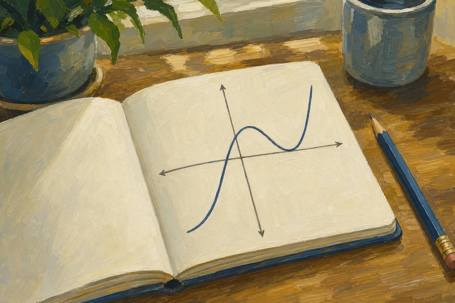
A cubic function graph is a smooth curve whose ends head in opposite vertical directions: it may climb all the way across, or rise, dip, and rise again. It represents a polynomial with highest power three, and even a curve that briefly flattens need not turn back.

That difference between flattening and turning explains much of the shape. This guide follows one working method: use the equation to anchor the curve, then read what happens between those anchors. The parent curve leads to transformations, intercepts, and turns, before a worked sketch shows how one horizontal line can reveal three solutions.

In This Article

• Recognize a Cubic Function
• Plot the Parent Curve
• Shift, Stretch, and Reflect the Curve
• Find Where the Curve Meets the Axes
• Locate Turning Points and the Inflection Point
• Build a Sketch From the Equation
• Use the Curve to Solve Equations
• Key Takeaways
• Frequently Asked Questions
• Read the Curve, Check the Solution

Recognize a Cubic Function

The equation behind that shape is

[ f(x)=ax^3+bx^2+cx+d,\qquad a\ne0, ]

where the letters represent real constants. The condition on (a) keeps the degree at three. Lower-power terms can be absent: (f(x)=4x^3-7) is still cubic. A quartic, by comparison, has degree four. Simplify before classifying an expression, since its highest-power terms might cancel.

The surviving terms compete to shape the curve. Near the origin, the constant or linear term may dominate what you see; far enough away, (ax^3) determines the direction. For (a>0), the left end falls and the right end rises. A negative (a) reverses those directions.

Those opposite ends belong to one continuous curve, with no holes or breaks, so it must cross the horizontal axis somewhere. The lower-power terms determine whether it makes further crossings along the way. Cubic functions share this end behavior without all sharing the same central shape.

Plot the Parent Curve

The parent curve, (y=x^3), strips away those competing terms. For this parent curve, each output is the product of three copies of the input: (x^3=x\times x\times x). At (x=2), squaring gives (4), while cubing gives (8): the cubic is already pulling away. On the negative side, the difference is sharper still, because ((-2)^3=-8), not (8).

That sign change places the negative half of the curve below the horizontal axis. The following coordinates show how quickly the outputs spread as you move away from zero.

Cubic graph coordinates: plotting the parent curve y = x³

Coordinate on y = x³	Plotting directions from (0, 0)	Parent cubic graph feature
(−2, −8)	2 units left; 8 units down	Lower-left branch in quadrant III
(−1, −1)	1 unit left; 1 unit down	Near-origin point in quadrant III
(0, 0)	At the intersection of the axes	Both intercepts; horizontal tangent; inflection point
(1, 1)	1 unit right; 1 unit up	Near-origin point in quadrant I
(2, 8)	2 units right; 8 units up	Upper-right branch in quadrant I

Draw a smooth curve through these points, measuring (x) horizontally and (y) vertically. From (x=1) to (x=2), the output jumps from (1) to (8); near zero, the curve almost lies flat. Yet it keeps increasing through the origin. Flat does not mean stopped, and it does not mean reversed.

The apparent steepness depends on the drawing's proportions. Use evenly spaced ticks on each axis and label both scales; the horizontal and vertical scales need not match. Compare coordinates, not the apparent narrowness of two drawings.

Shift, Stretch, and Reflect the Curve

A shift moves the entire parent curve without changing its shape. Its flat middle can sit above the axis or to the right of the origin. A vertical stretch pulls points farther from the horizontal line through that middle, making the branches look steeper; compression draws them toward it.

Shifts, stretches, and reflections of the parent curve (y=x^3) have the form

[ y=a(x-h)^3+k,\qquad a\ne0. ]

Not every cubic can be written in this form.

Here the inflection point is ((h,k)). Because the bracket contains (x-h), a positive (h) moves the curve right. Thus (y=(x-4)^3+2) moves it four units right and two units up.

The coefficient controls the stretch: (|a|>1) stretches vertically, while (0<|a|<1) compresses. A negative value also reflects the parent curve across the (x)-axis before translation. For example, (y=-2(x-1)^3+3) decreases from left to right, with its flat middle at ((1,3)).

To place individual points, transform a parent coordinate ((u,v)) into ((u+h,av+k)). The rule makes one detail visible: (a) multiplies the old output, not the vertical shift. Add (k) afterward.

Find Where the Curve Meets the Axes

A curve can slice through the horizontal axis or bounce back from it. Both happen in

[ f(x)=(x+2)(x-1)^2. ]

At (x=-2), the factor (x+2) changes sign while the squared factor stays positive nearby. The curve crosses at ((-2,0)). Around (x=1), the squared factor stays positive on either side and the other factor stays positive too. The curve reaches ((1,0)), then returns to the same side of the axis.

The repeated factor explains the bounce. Its repetition is called the root's multiplicity: an odd multiplicity gives a crossing, and an even multiplicity gives a touch without crossing. A triple root crosses with a horizontal tangent. Consequently, cubic graphs can have one, two, or three distinct real (x)-intercepts.

To find those intercepts, set

[ ax^3+bx^2+cx+d=0. ]

Factoring lets you use the zero-product rule, as in the example above; otherwise, graphical or numerical methods can locate approximate roots. Report intercepts as coordinate pairs. The vertical intercept requires only (x=0), giving ((0,d)) in general and ((0,2)) for this example.

Locate Turning Points and the Inflection Point

Every cubic has a center of half-turn symmetry: rotate its graph through (180°) about the inflection point, and the curve fits itself again. This point marks a change in bending, not necessarily a change in direction. Its horizontal coordinate is

[ x_{\mathrm{inf}}=-\frac{b}{3a}. ]

Substitution into the original function supplies its height. Consider (f(x)=x^3-6x^2+9x+1). The two turns, when present, sit on opposite sides of that center and correspond under the half-turn.

To locate turns precisely, differentiation gives

[ f'(x)=3ax^2+2bx+c. ]

This derivative measures slope. Setting it equal to zero finds stationary points, where the tangent is horizontal. A turning point must also reverse the direction of travel: increasing becomes decreasing, or decreasing becomes increasing.

For the example above, the derivative is (3(x-1)(x-3)). The stationary inputs are (1) and (3); the original function gives a local maximum at ((1,5)) and a local minimum at ((3,1)). These are nearby highs and lows, not absolute extremes of the unbounded curve.

In general, (b^2-3ac) decides how many stationary points exist. A positive value gives two turning points, at

[ x=\frac{-b\pm\sqrt{b^2-3ac}}{3a}. ]

A zero value gives one stationary inflection, with no turn; a negative value gives no stationary points. In either case, the curve still changes its bending at its inflection point. That point need not have a horizontal tangent: (y=x^3+x) has slope (1) there.

Build a Sketch From the Equation

For (y=x^3-3x), the cubic term promises rising behavior at the far right, but the negative linear term interrupts that rise in the middle. Factoring gives (x(x^2-3)). Setting this equal to zero gives (x=0,\pm\sqrt3), so the crossings are ((-\sqrt3,0)), ((0,0)), and ((\sqrt3,0)). The origin is also the vertical intercept.

The crossings anchor the sketch, but they leave a question: how high and low does the curve go between them? Differentiating gives (3x^2-3). Its zeros are (-1) and (1); the function has a local maximum at ((-1,2)) and a local minimum at ((1,-2)). The inflection point is the origin.

Plot those points before connecting them. Without calculus, extra coordinates on either side of a suspected turn can support an approximate sketch, though they do not establish its exact location. A cubic graph should still be drawn as a smooth curve, not as straight segments joining sampled points; arrowheads show its continuation beyond the drawing.

The completed curve rises through the left crossing to a local maximum, sweeps downward through the origin, bottoms out at ((1,-2)), and climbs through the right crossing. Its central stroke slopes down even though its ends establish an overall upward passage. That is the S-shape the equation's competing terms create.

Use the Curve to Solve Equations

The same S-curve can give three answers to one question. Draw (y=1) across the sketch of (y=x^3-3x): it cuts the left rising branch, the descending middle, and the right rising branch. Their horizontal coordinates solve

[ x^3-3x=1, ]

giving approximately (-1.53), (-0.35), and (1.88). One equation has three solutions because the curve reaches the same height on three separate passages.

Those passages must all fit in the displayed window. Include both turns when choosing the range; a view confined to the right branch hides two answers. For any equation (f(x)=m), the horizontal line (y=m) supplies the required height. When (m=0), that line is the horizontal axis itself.

A comparison between functions works the same way. The intersection inputs of (y=f(x)) and (y=g(x)) solve (f(x)=g(x)). Alternatively, graph (y=f(x)-g(x)) and read its zeros. Interpreting the equation of a cubic graph visually connects an algebraic equality to a shared position on the page.

Key Takeaways

• Classify the simplified equation before choosing a familiar curve shape.
• Use the leading coefficient to orient the ends, not to predict every movement between them.
• Distinguish a crossing from a touch by examining the root's multiplicity.
• Separate a horizontal tangent from a genuine reversal of direction.
• Read solutions as intersection inputs, accounting for every visible branch.

Frequently Asked Questions

The easiest shape to misread is the one with no turns: it can flatten, or even change its bending without ever becoming horizontal. These questions separate that behavior from the more conspicuous two-turn curve.

What Is a Cubic Function?

A cubic function is a polynomial of degree three, such as (f(x)=2x^3-x+6). Its domain and range are both all real numbers: neither the allowed inputs nor the available outputs have a finite boundary.

What Is a Cubic Graph?

A cubic graph is the set of coordinate pairs belonging to a cubic function. Every vertical line meets it exactly once because each input has one output. A horizontal line can meet it more than once because different inputs can share an output.

Can a Cubic Curve Have No Turning Points?

Yes; (y=x^3+2x) increases everywhere and has no turning points. Its slope, (3x^2+2), is always positive, so it has no horizontal tangent either. Unlike the parent curve, it passes through its change of bending without even flattening.

Why Do Some Cubic Curves Cross the x-Axis Only Once?

Some cubic curves cross only once because any turns they have do not bring them back across the axis. For example, (y=x^3-3x+4) has both turns above the axis and a single crossing on the left branch. Its other two roots are nonreal.

Can a Cubic Curve Touch the x-Axis Without Crossing It?

Yes; a double root makes a cubic curve touch the axis without crossing there. The function keeps the same sign on either side of that root. A separate crossing occurs elsewhere, as in the factored example above.

How Can You Check Whether a Graph-Based Solution Is Accurate?

Substitute the estimated input into the original equation and compare the two sides. Keep extra decimal places during calculation, and refine the estimate if the difference exceeds the required tolerance. Graph readings remain approximate; use algebra where possible when an exact answer is required.

Read the Curve, Check the Solution

Begin by deciding what you need from the graph. For a rough shape, intercepts and a few coordinates may suffice; for exact turning points, use differentiation. For an equation's solutions, identify the height or second function whose intersections matter.

The revealing detail in (y=x^3-3x) is its downward middle stroke. Without that reversal, the line (y=1) could not meet this curve three times. Each intersection answers the same question at a different input. A sketch makes those answers visible together, while substitution tests each one separately. That is the useful division of work: let the curve show how many answers you need to account for, and let calculation establish how accurately you have found them.