A bimodal histogram shows two prominent peaks: observations cluster around two different ranges, with fewer observations between them. That matters when one chart combines two operating conditions and an overall average hides the difference. A component-test example shows how to read the separation and decide what to investigate next.

In This Article

• What the Two Peaks Tell You
• A Two-Peak Example You Can Read
• Check Whether the Shape Holds Up
• Look for Differences Behind the Peaks
• Why One Average Can Mislead
• Choose Your Next Analysis
• Key Takeaways
• Frequently Asked Questions
• Investigate What Separates the Peaks

What the Two Peaks Tell You

Suppose you measure how long a component takes to complete a test. Readings accumulate near 15 milliseconds and again near 25 milliseconds, with relatively few in between. Those concentrations are the peaks: each represents a range of common durations, not necessarily a single tall bar. In a bimodal distribution histogram, the two high-frequency regions make that separation visible.

The intervals used to draw the chart affect how precisely you can locate each peak. A bar covering 14 to 16 milliseconds tells you how many measurements fall within that interval; without the raw readings, it does not tell you their exact values.

A unimodal histogram has one broad concentration; bimodal histograms have two. Read the neighboring bars together. A supported second concentration matters; a stray outlier does not make a second peak.

A Two-Peak Example You Can Read

Consider these constructed component-test durations, measured in milliseconds. They illustrate a pattern; they are not results from a reported experiment:

11, 13, 13, 13, 15, 15, 15, 15, 15, 15, 15, 17, 17, 17, 17, 19, 21, 23, 23, 23, 23, 25, 25, 25, 25, 25, 25, 25, 25, 27, 27, 27, 29.

The histogram plots all 33 observations in equal-width intervals. Duration runs across the horizontal axis; frequency runs up the vertical axis.

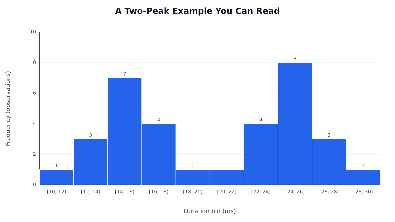
The notation [10, 12) includes 10 but excludes 12, so a reading on a shared boundary belongs to only one bin. This histogram has local peaks in the intervals containing 15 and 25 milliseconds. These are not two equally frequent raw values: 15 occurs seven times and 25 eight times. NIST defines the sample mode as the value occurring most frequently. By that definition, 25 milliseconds is the sample’s single mode. The grouped bars locate the two concentrations only within their intervals.

A valley need not be empty. Nor must the peaks match. The chart still has two clear concentrations.

Those concentrations also need not form a symmetric outline. A bimodal histogram can be skewed, with a longer outer tail on one side. Peak count describes modality; the balance of the shape describes symmetry. Neither property supplies the missing test records that would explain why these durations differ.

Check Whether the Shape Holds Up

Change the bins before explaining the peaks. Here is the same dataset regrouped into wider intervals; the counts show exactly what changes:

Bin Width	Intervals in Milliseconds	Counts, in Interval Order
3 ms	[10,13), [13,16), [16,19), [19,22), [22,25), [25,28), [28,31)	1, 10, 4, 2, 4, 11, 1
4 ms	[10,14), [14,18), [18,22), [22,26), [26,30)	4, 11, 2, 12, 4

The lower and upper concentrations remain. Wider bars combine neighboring readings; they do not create additional measurements.

Moving the boundaries changes the picture again. The underlying values have not moved. A width chosen only to sharpen a preferred story is a poor basis for that story.

A dot plot exposes the individual values without bin boundaries. Use it beside the histogram, especially for a small sample where a few readings can reshape a bump. A density curve offers another view, although its bandwidth controls how much detail gets smoothed away.

Also inspect the recording rules. Whole-millisecond rounding can pile readings at repeated values; recording or plotting below-limit observations at the detection limit can pile them at that limit. A peak at that limit calls for a measurement investigation before a process explanation.

Look for Differences Behind the Peaks

For a concrete factory-floor investigation, suppose the component tests cover a day shift and a night shift. The question is whether the longer durations belong mainly to one shift. The supplied dataset has no shift labels, so this is a worked investigation to pursue, not a finding already contained in the numbers.

Attach the recorded shift to each test, then draw separate histograms with matching axes and bin boundaries. If day-shift readings cluster near 15 milliseconds and night-shift readings near 25, the combined chart has exposed a difference between shifts. If each shift contains both peaks, shift membership does not explain the separation. That result redirects the investigation immediately.

A shift difference gives you somewhere specific to look. Suppose the night shift also uses a different product version. Compare that version across shifts before blaming shift practice: otherwise, a product difference could masquerade as a staffing effect. The useful comparison holds one condition steady while examining the other.

Collection order adds information the histogram discards. Plot the durations in sequence and mark the shift handover. A sustained jump at the handover points toward a changed condition; high and low readings alternating within both shifts point toward something recurring during production. Use that distinction to choose which operating records to examine next.

Why One Average Can Mislead

The 33 durations sum to 665 milliseconds, giving an overall mean of approximately 20.15 milliseconds. That falls in the low-frequency valley between the peaks, rather than near either concentration. This is the central reporting problem with bimodal data: a correct calculation can describe an uncommon result.

On the factory floor, that pooled mean could become a planning assumption. In the shift scenario, scheduling every test around it would leave too little time for the slower condition and excess time for the faster one. The arithmetic is sound; its application is wrong. A condition-specific estimate answers the scheduling question more directly.

The overall standard deviation of the combined data can create a different cost. It includes the separation between the concentrations as well as variation within them. Suppose a team treats that overall spread as evidence that the faster shift is unstable: it might spend time adjusting an already consistent operation while leaving the shift difference untouched.

Keep the histogram beside the summary. When records support separate groups, report their centers and spreads with their sample sizes; without those records, describe the observed clusters without assigning them to populations.

Choose Your Next Analysis

Use labels first when reliable labels exist. For the shift investigation, comparing recorded day and night tests is more interpretable than asking a model to reconstruct groups you already know. For a descriptive report, the histogram and raw-value display may be enough.

Consider a mixture model when group membership is unknown and estimating overlapping components would help answer your question. Treat those fitted components as a model of the measurements, not as discovered machines or shifts. A model can separate durations mathematically without identifying their operational source.

For prediction, decide which conditions future tests will represent. A single normal model describes a unimodal distribution, so it cannot directly represent two separated concentrations. A mixture may suit a future stream containing both conditions; a group-specific model may suit a known condition. Choose according to the prediction task, not the visual appeal of a fitted curve.

Formal tests of multimodality can supplement the plots when you need a statistical assessment of the shape. Their interpretation depends on sample size and assumptions. They answer a shape question, not the factory-floor question of what changed. Judge any process intervention against the performance requirement, not whether it produces a tidier histogram.

Key Takeaways

• Read a peak as a concentration across neighboring bars; do not count isolated tall rectangles.
• Use the regrouped example as a reminder to test both bin width and starting boundary.
• Keep shift labels and collection order attached to readings so the chart can lead to a useful comparison.
• Match summaries and prediction models to the conditions your decision concerns.

Frequently Asked Questions

The distinctions below help when the chart’s shape is less clear than the worked example.

What’s the Difference Between Bimodal and Multimodal?

Bimodal specifies exactly two modes; multimodal includes any pattern with more than one mode. Use “bimodal” when two concentrations are the feature you want to describe, and “multimodal” when discussing the broader category.

Can a Bimodal Histogram Be Skewed?

Yes, a bimodal histogram can have a longer tail on one side. Describe that asymmetry separately from the two concentrations; skewness does not turn two peaks into one.

How Do You Know If It’s Unimodal or Bimodal?

Look for one broad concentration or two concentrations separated by lower frequencies. Then compare sensible bin choices and the individual readings. If a weak second bump vanishes with small plotting changes, leave the classification tentative.

What Is Bimodal Distribution?

A bimodal distribution has two modes, or local peaks in probability density or probability mass. A sample histogram provides evidence about that structure, but the population’s shape remains an inference from the observations.

Do the Two Peaks Have to Be the Same Height?

No, the two peaks can have different heights. A narrow concentration can produce a tall peak without containing more observations overall, so compare the full regions when judging their relative sizes.

Does a Two-Peak Pattern Prove That Two Populations Were Combined?

No, two peaks do not prove that two populations were combined. Different operating states within one process, measurement effects, or sampling variation can produce the pattern. Conversely, combined populations may overlap enough to show only one peak.

Investigate What Separates the Peaks

For the next component-test run, record both shift and product version alongside every duration, preserving collection order. Compare the same product version across shifts using histograms with matching axes and bin boundaries. If each shift still contains both peaks, shift membership does not explain the separation; examine other operating records before choosing an intervention.