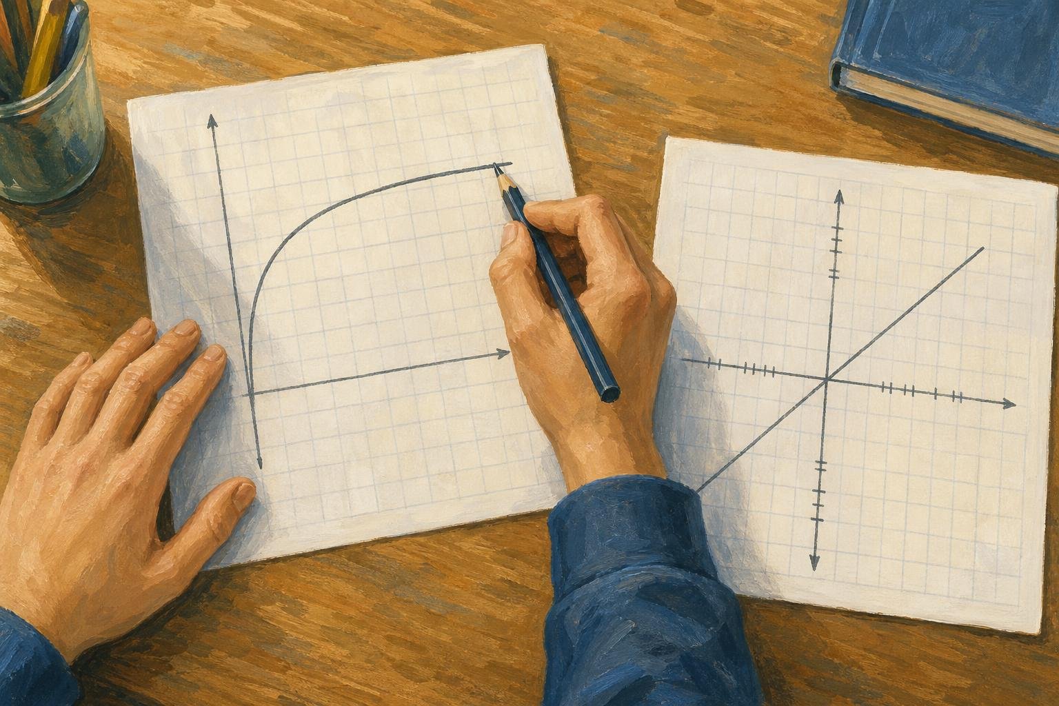
A logarithmic graph can put equal ratios at equal distances: 10 to 100 takes as much space as 100 to 1,000. That visual trick comes from logarithmic axes; plotting a logarithmic function on ordinary axes is a different operation.

In This Article

• Tell the Function From the Axes
• Read Values on a Log Scale
• Plot a Logarithmic Function
• Shift, Reflect, and Stretch the Curve
• Find an Equation From Points
• Recognize Straight Lines on Log Axes
• Key Takeaways
• Frequently Asked Questions
• Start With the Argument and Asymptote

Tell the Function From the Axes

Suppose three equally spaced marks read 1, 10, and 100. Read them as ordinary spacing and you might call the middle value halfway between the endpoints. It isn't: that would be 50.5. The labels overturn the picture.

A logarithmic function instead reverses exponentiation: y = log_b(x) means x = b^y, with b > 0 and b ≠ 1. Thus log₂(8) = 3 because 2³ = 8. The natural logarithm, ln(x), uses Euler’s number, e. A semilog chart has one logarithmic axis; a log–log chart has two. Keep the function and the axis spacing separate throughout.

Read Values on a Log Scale

On a base-10 axis, the equally spaced labels 1, 10, 100, and 1,000 each mark a tenfold increase. Between 10 and 100, ticks for 20–90 crowd progressively closer together.

Halfway between 10 and 100 is √(10 × 100) ≈ 31.6, not 55: each half covers the same ratio, √10. To read a complete point, check each axis separately. With a logarithmic x-axis and a linear y-axis, a point halfway between x = 10 and x = 100 and level with y = 2 has coordinates approximately (31.6, 2).

A standard log graph cannot display zero or negative values on its logarithmic axis.

For a real example, USGS’s “Monitoring location pages and log scale” shows Long Branch near Annandale, Virginia, station 01654500, March 24–April 23, 2025. Time is linear; discharge is logarithmic. The April 7 peak reads approximately 60 ft³/s, between the labeled 50 and 100 ticks. To interpolate, measure the fraction f upward from 50 toward 100, then calculate 50 × (100/50)^f: one-quarter gives about 59.5 ft³/s. This is a visual estimate, not an exact recorded value.

Plot a Logarithmic Function

The shortcut for learning how to graph log functions is to choose outputs first. For y = log₂(x), outputs −1, 0, 1, and 2 give x = 2^y, producing (½, −1), (1, 0), (2, 1), and (4, 2). Plot them on linear axes and join them smoothly.

This logarithm graph has domain x > 0 and range all real numbers. Compare the first and last rows below: a base above 1 gives an increasing curve; a base between 0 and 1 reverses its direction.

Logarithmic function	Point where y = 1	Change in y when x doubles	Change in y when x increases tenfold
y = log₂(x)	(2, 1): base 2	+1	+log₂(10) ≈ +3.322
y = log₃(x)	(3, 1): base 3	+log₃(2) ≈ +0.631	+log₃(10) ≈ +2.096
y = ln(x)	(e, 1), e ≈ 2.718: base e	+ln(2) ≈ +0.693	+ln(10) ≈ +2.303
y = log₁₀(x)	(10, 1): base 10	+log₁₀(2) ≈ +0.301	+1
y = log₁⁄₂(x)	(½, 1): base ½	−1	−log₂(10) ≈ −3.322

Either way, the logarithmic function graph approaches its vertical asymptote, x = 0. It never touches it.

Shift, Reflect, and Stretch the Curve

The minus sign is the trap: log₂(−x) and −log₂(x) send the same reference point in different directions. Inside, it reflects (2, 1) to (−2, 1), requiring x < 0. Outside, it reflects that point to (2, −1), keeping x > 0.

For the broader form y = a log_b(x − h) + k, move a parent point (u, v) to (h + u, av + k). For b > 0 and b ≠ 1, the condition x − h > 0 sets the domain; x = h is the vertical asymptote provided a ≠ 0. The table keeps the other operations available without obscuring that inside/outside distinction.

Curve transformation	Logarithmic equation	Image of reference point (2, 1)	Domain	Vertical asymptote	Curve direction as x increases
Original curve	y = log₂(x)	(2, 1)	x > 0	x = 0	Increasing
Shift right 3 units	y = log₂(x − 3)	(5, 1)	x > 3	x = 3	Increasing
Shift left 3 units	y = log₂(x + 3)	(−1, 1)	x > −3	x = −3	Increasing
Shift up 2 units	y = log₂(x) + 2	(2, 3)	x > 0	x = 0	Increasing
Shift down 2 units	y = log₂(x) − 2	(2, −1)	x > 0	x = 0	Increasing
Reflect across the y-axis	y = log₂(−x)	(−2, 1)	x < 0	x = 0	Decreasing
Reflect across the x-axis	y = −log₂(x)	(2, −1)	x > 0	x = 0	Decreasing
Vertical stretch by factor 3	y = 3log₂(x)	(2, 3)	x > 0	x = 0	Increasing
Vertical compression by factor ½	y = ½log₂(x)	(2, ½)	x > 0	x = 0	Increasing

Find an Equation From Points

A curve hides its formula but leaves clues: an asymptote at x = 3 and points (4, 0) and (5, 2). Assuming y = a log₂(x − h) + k, the boundary reveals h = 3.

Now (4, 0) makes the logarithm zero, exposing k = 0. At (5, 2), the logarithm equals one, exposing a = 2. The recovered equation is y = 2 log₂(x − 3); other plotted points can test the fit. Without an assumed model, those clues don't settle the formula.

Recognize Straight Lines on Log Axes

For an ideal point sound source of fixed power in free space, spherical spreading without absorption gives intensity proportional to inverse distance squared: I ∝ r⁻². On log–log axes, that relationship becomes a straight line of slope −2.

The general rule is y = A x^k: log(y) = log(A) + k log(x), for A > 0 and x > 0. Using the same base on both axes makes the slope k. For exponential data, y = A b^x gives log(y) = log(A) + x log(b), with A > 0 and b > 0; only the y-axis needs logarithmic spacing. These logarithmic graphs turn multiplicative relationships into readable slopes.

Key Takeaways

• Let axis labels decide what equal distances mean.
• Use convenient outputs to generate plotting points.
• Treat an inside minus sign differently from an outside one.
• Choose a model before recovering its coefficients.

Frequently Asked Questions

How do you know if a graph is logarithmic or exponential?

On linear axes, basic logarithmic curves have vertical asymptotes; basic exponential curves have horizontal ones. For example, y = log₂(x) passes through (1, 0) and approaches x = 0. A straight line alone proves neither: its axes may be logarithmic.

Is a logarithmic or linear chart better?

Linear charts suit absolute differences; logarithmic charts suit ratios, such as successive tenfold increases. Choose the latter when small positive values would otherwise be compressed near the axis, but not when you need to display zero or negative values.

How do you read a logarithmic graph?

Read each coordinate using its own axis scale; one may be linear while the other is logarithmic. Between labeled powers, use ratio-based positioning: halfway from 10 to 100 is √(10 × 100) ≈ 31.6, not 55.

How does a logarithmic function differ from a linear function?

For a linear function, equal increases in x produce equal changes in y. For y = log_b(x), multiplying x by a fixed positive factor produces a fixed change in y instead: doubling x changes y by log_b(2). Thus y = log₂(x) gains 1 whenever x doubles.

Can two logarithmic equations with different bases describe the same curve?

Yes, adjusting the coefficient can compensate for changing the base. For example, log₂(x) = ln(x)/ln(2), giving identical coordinates throughout their shared domain, x > 0. Without that coefficient adjustment, changing the base generally changes the curve.

Start With the Argument and Asymptote

Before drawing a log function graph, inspect the argument inside the logarithm. Its positivity condition tells you where points are allowed, so a beautifully drawn curve on the wrong side is still wrong. In the recovered equation, x − 3 puts the entire curve to the right of its boundary.

Then use the supplied points as an independent test: a correct boundary cannot rescue incorrect coordinates. For a data chart, the first choice is different. Decide whether an absolute change or a proportional change answers your question, then choose the spacing that preserves that comparison. Don't let a straight-looking line make the decision for you.

Read the axes before trusting the shape.