Blog

David Martinez•November 5, 2026·November 9, 2026•10 min read

Quadratic Graph: One Worked Example, From Curve to Roots

Table of Contents

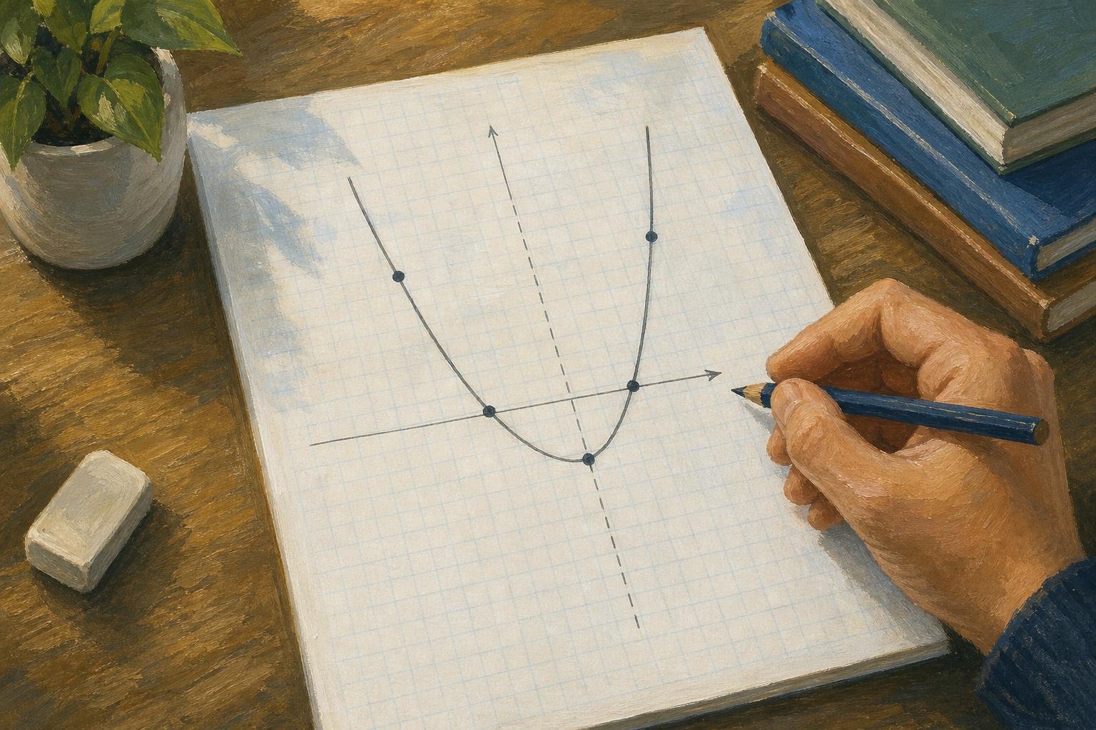
A quadratic graph is a parabola: a smooth curve that opens upward or downward. To plot one, find its vertex and symmetry line, calculate a few matching points on either side, and locate any intercepts; its real roots are the x-values where it meets the x-axis.

This article connects those steps through one worked example, then explains how transformations change the curve and how to recover an equation from a graph. The same approach works throughout: identify a feature in the equation, calculate its position, and use it to guide your sketch.

What Makes the Curve a Parabola?

A quadratic function has the form

[ y=ax^2+bx+c,\qquad a\ne0. ]

The highest power of (x) is two. The condition (a\ne0) matters: without the squared term, the equation describes a straight line or a constant function. In the Cartesian coordinate system, each point ((x,y)) pairs an input with its output. Plotting these pairs produces the quadratic function graph, called a parabola.

The coefficient (a) determines the opening direction. When (a>0), the curve opens upward and has a lowest point. When (a<0), it opens downward and has a highest point. That turning point is the vertex. The phrase “positive quadratic graph” usually describes the upward-opening case; it does not mean every output is positive.

These features provide a useful checklist for reading an equation or an existing graph.

Quadratic graph features: formulas and a worked example

Quadratic graph feature	Rule for y = ax² + bx + c, a ≠ 0	Example: y = 2x² − 8x + 6	What to read from the graph
Opening direction	a > 0: upward; a < 0: downward	a = 2; opens upward	Upward: minimum; downward: maximum
Vertex	h = −b/(2a); k = ah² + bh + c	Vertex: (2, −2)	Turning point at x = 2, y = −2
Axis of symmetry	Vertical line x = −b/(2a)	x = 2	Points at equal horizontal distances from x = 2 have equal heights
x-intercepts (real roots)	Solve ax² + bx + c = 0	2(x − 1)(x − 3) = 0; intercepts (1, 0), (3, 0)	Where the curve meets the x-axis
y-intercept	Set x = 0; point is (0, c)	(0, 6)	Where the curve meets the y-axis
Number of x-intercepts	D = b² − 4ac; D > 0: two; D = 0: one; D < 0: none	D = 64 − 48 = 16; two x-intercepts	Two crossings, one touch, or no contact with the x-axis
Domain	All real x-values	−∞ < x < ∞	The curve extends indefinitely left and right
Range	Vertex height k: y ≥ k if a > 0; y ≤ k if a < 0	y ≥ −2	No point lies below y = −2 in this example

For the quadratic graph y = 2x² − 8x + 6, the parabola opens upward, has vertex (2, −2) and symmetry axis x = 2, crosses the axes at (1, 0), (3, 0) and (0, 6), accepts every real x-value and has outputs y ≥ −2.

The curve itself is important. Although you might encounter the label “quadratic line graph,” a parabola is not made from straight segments connecting calculated points. Those points are samples from a continuous curve, and your sketch should bend smoothly through them.

Find the Vertex and Axis of Symmetry

For a quadratic written in standard form, the vertex formula gives its horizontal position:

[ h=-\frac{b}{2a}. ]

Substitute (h) into the function to find the vertical coordinate (k=f(h)). The vertex is ((h,k)), and the vertical line (x=h) is the axis of symmetry. Points equally far to the left and right of this line have equal outputs. That property reduces the arithmetic needed for a sketch.

Use this quadratic graph example:

[ y=2x^2-8x+6. ]

Here (a=2), (b=-8), and (c=6). Therefore,

[ h=-\frac{-8}{2(2)}=2, \qquad k=2(2)^2-8(2)+6=-2. ]

The vertex is ((2,-2)), with symmetry line (x=2). Because the squared-term coefficient is positive, this vertex is a minimum.

Be careful with the sign of (b). In this example, (b) is the entire coefficient (-8), not (8). Writing the substitution before simplifying helps prevent a misplaced vertex. Also distinguish the point from the line: ((2,-2)) names one location, while (x=2) includes every point on the vertical symmetry line.

Plot Points on Both Sides

With the vertex located, choose nearby x-values on both sides of its symmetry line. For the example, use (x=0,1,2,3,4). Substitution gives the corresponding y-values (6,0,-2,0,6). The matching outputs at equal distances from (x=2) provide a built-in arithmetic check. If your values do not match, revisit the substitutions before drawing.

A table organizes those calculations and makes the symmetry easier to see. To simplify substitution, rewrite the same equation by completing the square:

[ 2x^2-8x+6=2(x^2-4x+4)-2=2(x-2)^2-2. ]

This equivalent expression is the vertex form used in the table below.

Quadratic graph: calculated values and points for a parabola

Input x	Calculation: y = 2(x − 2)² − 2	Output y	Point to plot	Parabola feature
0	2(−2)² − 2 = 6	6	(0, 6)	y-intercept; mirrors (4, 6)
1	2(−1)² − 2 = 0	0	(1, 0)	Left x-intercept; mirrors (3, 0)
2	2(0)² − 2 = −2	−2	(2, −2)	Vertex; minimum y-value
3	2(1)² − 2 = 0	0	(3, 0)	Right x-intercept; mirrors (1, 0)
4	2(2)² − 2 = 6	6	(4, 6)	Mirrors (0, 6) across x = 2

For the quadratic graph y = 2(x − 2)² − 2, inputs 0, 1, 2, 3 and 4 give outputs 6, 0, −2, 0 and 6, forming five plotting points symmetric about x = 2.

Plot the five coordinate pairs on labeled axes with consistent spacing. The scale does not have to be identical on both axes, but each axis must keep its own spacing uniform. Mark the vertex clearly, then draw a smooth curve through the points. Both branches should continue upward beyond the plotted samples, with arrowheads showing that they extend.

The point at (x=0) is especially useful because it lies on the y-axis. In standard form, substituting zero leaves (y=c), so the y-intercept is always ((0,c)). If your drawing misses that point, either a calculation or the sketch needs correction. Extra points help near a sharp turn, but they should support the curve, not turn it into a polygon.

Describe the Domain, Range, and Shifts

A quadratic function accepts every real input, so its domain is all real numbers, written ((-\infty,\infty)). Its range depends on the vertex and opening direction. For vertex ((h,k)), the range is (y\ge k) when (a>0), and (y\le k) when (a<0). The equality is included because the vertex belongs to the curve. For the worked example, the range is (y\ge-2).

Vertex form makes this boundary and the graph’s transformations easier to read:

[ y=a(x-h)^2+k. ]

Starting with the parent graph (y=x^2), the expression (x-h) shifts the vertex horizontally to (x=h), while (k) shifts it vertically. A positive (h) moves the vertex right; a negative (h) moves it left. The sign inside the parentheses therefore needs careful reading.

The factor (|a|) scales vertical distances from the vertex’s horizontal level. If (|a|>1), the parabola appears narrower than the parent graph; if (0<|a|<1), it appears wider. A negative (a) also reflects the parent curve across the x-axis before translation.

For example, (y=-\tfrac12(x+3)^2+4) has vertex ((-3,4)). Its branches open downward and appear wider than those of the parent graph. These features can guide a sketch before you calculate any additional points.

Find the Roots and Count the Intercepts

To use a quadratic equation graph to solve (ax^2+bx+c=0), locate its x-intercepts. At each one, the output is zero. Read the horizontal coordinate as the root, not the entire ordered pair. For the worked example, factoring gives

[ 2x^2-8x+6=2(x-1)(x-3). ]

The zero-product property gives roots (x=1) and (x=3). These are exact results. A crossing read from a rough sketch may only provide an estimate, especially when it falls between grid marks.

When factoring is difficult, use the quadratic formula:

[ x=\frac{-b\pm\sqrt{b^2-4ac}}{2a}. ]

The expression under the square root is the discriminant, (\Delta=b^2-4ac). If (\Delta>0), there are two distinct real roots and two x-intercepts. If (\Delta=0), there is one repeated real root. If (\Delta<0), there are no real roots and no x-intercepts.

For the worked example, the discriminant is (16), consistent with the two crossings already found. By comparison, (y=x^2+1) has discriminant (-4): its curve remains above the x-axis. It still has complex roots, but those are not x-intercepts on the real coordinate plane. This distinction keeps “no real roots” from being confused with “no solutions of any kind.”

Recover an Equation From a Graph

You can also work backward from a graph. If the vertex is visible, insert its coordinates into vertex form, leaving (a) unknown. Then substitute one other point on the curve to determine the missing coefficient. That point must differ from the vertex: using the vertex again makes the squared term zero and supplies no information about the opening.

For example, suppose a graph has vertex ((2,-2)) and passes through ((0,6)). Write

[ y=a(x-2)^2-2. ]

Substituting the other point gives (6=4a-2), so (a=2). Expanding the completed equation recovers the standard-form expression used earlier. This also shows why knowing only the vertex is insufficient: many parabolas share a turning point but have different widths or opening directions.

If two roots are easier to read, use factored form instead:

[ y=a(x-r_1)(x-r_2). ]

For instance, roots (-2) and (4) give (y=a(x+2)(x-4)). If the graph also passes through ((0,-8)), substitution gives (-8=-8a), so (a=1). The additional point cannot be either root, because that would only produce (0=0). When coordinates come from an approximate drawing, treat the recovered equation as approximate too.

Key Takeaways

A quadratic function has a nonzero squared-term coefficient and a parabolic graph.
The sign of (a) determines whether the vertex is a minimum or maximum.
The vertex lies on the symmetry line (x=-b/(2a)).
Symmetric table values help produce a reliable, smooth sketch.
Real roots are the x-coordinates where the curve meets the x-axis.

Frequently Asked Questions

Does a parabola stop at the last point in a table?

No. A table contains selected samples, not endpoints; for example, a row ending at (x=4) does not exclude (x=5). The curve continues beyond the listed points unless an application explicitly restricts the domain.

Must the vertex have whole-number coordinates?

No; fractions and irrational numbers can occur. For example, (y=x^2-x) has vertex ((\tfrac12,-\tfrac14)), so rounding to nearby whole numbers would move the turning point incorrectly.

Can the vertex also be the y-intercept?

Yes, when the vertex has horizontal coordinate zero. For example, (y=3x^2+5) has vertex and y-intercept at ((0,5)), so its symmetry line is the y-axis.

Why can a parabola cross the x-axis twice but the y-axis only once?

The equation (f(x)=0) can have two different inputs, each producing an x-axis crossing. The y-axis requires the single input (x=0), and a function assigns that input only one output.

Can two different quadratic functions have the same roots?

Yes. For example, (y=(x-1)(x-3)) and (y=2(x-1)(x-3)) have the same roots but different vertical scales. Roots alone do not determine the coefficient multiplying the factors.

How can you recognize a repeated root from the curve?

The vertex touches the x-axis without crossing it. For example, (y=(x-2)^2) has repeated root (x=2); nearby outputs on both sides remain positive.

Start With the Vertex and Symmetry

When you face an unfamiliar quadratic, choose the form that makes its useful features easiest to read. Standard form supports the vertex calculation; vertex form reveals the turning point directly. Factored form is especially helpful when your immediate goal is finding roots.

For the worked example, use the calculated vertex as your anchor and let symmetry guide the remaining points. Draw a smooth curve, then compare its intercepts with the algebraic results. If they disagree, return to the substitutions before changing the curve by eye. Quadratic graphs become manageable when each visible feature has a calculation behind it. Keep exact values when algebra supplies them, and label values read from a rough drawing as estimates.