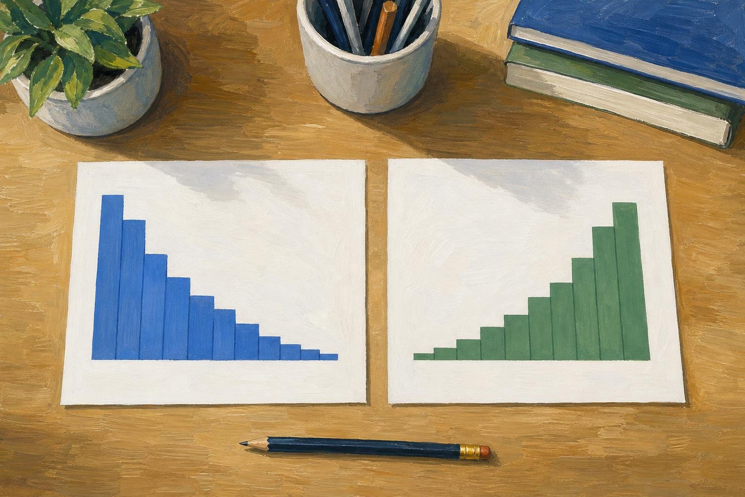
A right-skewed histogram has a longer tail toward larger values; a left-skewed histogram has a longer tail toward smaller values. The tallest bars usually sit toward the opposite side, so naming the skew from the peak reverses the answer.

To distinguish skewed right vs left, read the numerical axis first and follow the thinner stretch of observations away from the main concentration. This guide uses that approach throughout: identify the tail in a right vs left skewed histogram, assess the evidence, and choose an interpretation that fits your question.

In This Article

• Read the Tail Before the Tallest Bars
• Connect the Shape to Familiar Examples
• Treat the Mean and Median as Supporting Evidence
• Make Sure Binning Has Not Changed the Story
• Measure Asymmetry Without Claiming More Than It Shows
• Choose Summaries and Methods for Your Question
• Key Takeaways
• Frequently Asked Questions
• Let the Tail Guide Interpretation

Read the Tail Before the Tallest Bars

A histogram groups numerical observations into intervals called bins. Bar height represents frequency when the vertical axis shows counts; the horizontal axis places smaller values on the left and larger values on the right. A tail is the thinner stretch extending away from the main concentration. In a right vs left skewed histogram comparison, right skew is called positive skew, while left skew is called negative skew. Those names describe asymmetry, not whether the observations themselves are positive or negative.

Each column is intended to represent an equal-width bin, with the labeled value marking its midpoint rather than a boundary.

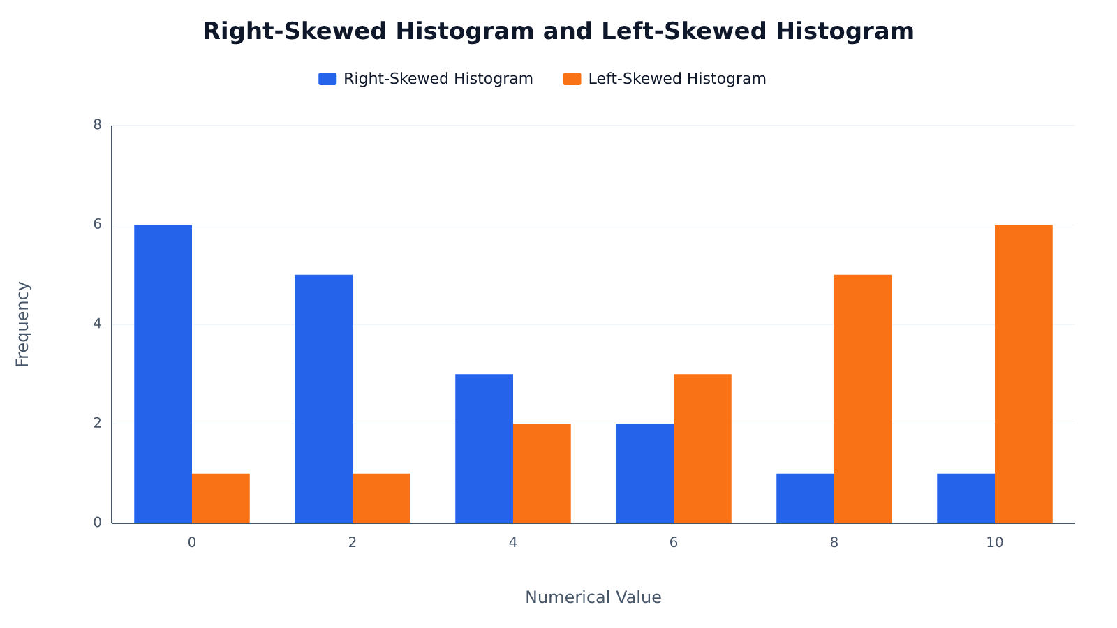
The right-hand plot concentrates observations at larger values, yet it is skewed left because its thinner extension runs toward smaller values. For a quick comparison of skewed left vs skewed right, use the tail as the deciding feature.

Right vs left skewed histogram: four checks for reading the shape

Histogram identification check	Right-skewed histogram	Left-skewed histogram
Tail-direction rule	Longer tail extends toward larger values (right)	Longer tail extends toward smaller values (left)
Observation-cluster check	Most observations cluster toward the lower-value side	Most observations cluster toward the higher-value side
Moment-based skewness clue	A coefficient > 0 supports right skew; interpret alongside the plotted shape	A coefficient < 0 supports left skew; interpret alongside the plotted shape
Mean–median heuristic	Mean is typically above the median; not a universal rule	Mean is typically below the median; not a universal rule

Connect the Shape to Familiar Examples

Income distributions commonly illustrate right skew. Many people earn incomes within a relatively concentrated range, while fewer earn much larger amounts. Those high incomes stretch the distribution’s upper end. In a right skewed distribution, the unusually large values can be far from the main group even though relatively few observations occupy that part of the graph. The tail shows how far those relatively few high incomes extend beyond the main group.

Scores on an easy test illustrate the opposite pattern. Suppose most students score close to the maximum, while a few receive substantially lower scores. A left skewed histogram would show tall bars near the upper end and a thinner extension toward lower scores. Every score could still be positive. The test’s upper limit also matters: students cannot extend the distribution beyond the maximum, but lower scores have room to stretch away from the main concentration. These are familiar patterns, not guarantees about every income sample or test.

Treat the Mean and Median as Supporting Evidence

Extreme observations affect the arithmetic mean because every value contributes directly to its calculation. The median depends on the middle position after sorting. In many simple, single-peaked distributions, the mean lies above the median under right skew and below it under left skew. This familiar ordering is useful supporting evidence, but it is not a definition. Multiple clusters or an unusual balance of observations can break the shortcut even when a moment-based skewness coefficient has a clear sign.

Two averages cannot establish skew direction on their own. Inspect the distribution and use the mean–median ordering only as supporting evidence.

Make Sure Binning Has Not Changed the Story

Bin width controls how much detail a histogram reveals. Narrow bins can expose gaps and local clusters, but they can also make a small sample look jagged. Wide bins merge nearby observations and may conceal an extension that looked important in a finer view. Bin boundaries matter too: shifting their starting points can divide one cluster across adjacent bars or gather it into a single taller bar. Neither choice changes the observations themselves.

For example, a few unusually large observations might occupy separate bars under narrow bins and share one bar under wider bins. Their numerical positions remain the same, but the apparent continuity of the tail changes. Compare a few reasonable bin widths and boundary positions while keeping the same horizontal scale. With a small sample, isolated bars and sampling noise do not necessarily establish a persistent population tail. A dot plot can help you see whether the apparent extension rests on several observations or one distant point.

Measure Asymmetry Without Claiming More Than It Shows

A skewness coefficient summarizes asymmetry numerically. A common moment-based version divides the average cubed deviation from the mean by the cube of the standard deviation, using consistent moment definitions. Cubing preserves the sign of each deviation and gives distant observations substantial influence. Positive values indicate positive moment skewness; negative values indicate negative moment skewness. Software may instead report a bias-adjusted sample version, so the estimator matters when comparing results, especially for small samples.

A coefficient near zero does not prove normality. A uniform distribution can be symmetric without having a bell shape, and a symmetric distribution can have two peaks. Skewness also does not establish tail weight: a symmetric distribution may place substantial probability far from its center. Keep asymmetry separate from questions about extreme-value frequency or normal-model fit. There is no universal coefficient cutoff that makes data acceptable for every analysis; the relevant standard depends on the method and the consequences of a poor fit.

Choose Summaries and Methods for Your Question

For right skewed data such as incomes, the median often answers what a typical person receives more directly than the mean. Pairing it with the interquartile range (IQR) describes the spread of the middle half of observations without letting the most extreme values dominate that summary. Yet the mean remains important when the question concerns an average per person or an aggregate total. A budget analysis and a description of a typical household may legitimately emphasize different summaries of the same distribution.

That difference in purpose also guides analysis. A skewed histogram does not automatically require a transformation. First identify what you want to estimate and which assumptions your method requires. Transforming values changes the scale and interpretation, so a more symmetric picture is not sufficient justification. In regression, distinguish the marginal histogram shown here from the conditional errors or outcome distribution specified by the model; they answer different questions.

Key Takeaways

• Name skew direction from the longer tail, not the tallest bars.
• Positive skew extends toward larger values; negative skew extends toward smaller values.
• The mean moves toward extreme observations, but familiar mean–median orderings are not universal.
• Skewness coefficients quantify asymmetry; they do not establish normality or explain tail weight.
• Choose summaries and methods that answer the analytical question; justify any transformation by its purpose and interpretation.

Frequently Asked Questions

What Does It Mean If a Histogram Is Skewed to the Right?

Its thinner extension reaches toward larger numerical values. The income example above shows why this can happen even when most observations lie toward the lower end. “Positive skew” is the alternative name for that direction.

Can a Distribution Contain Only Positive Values and Still Have Negative Skew?

Yes. Negative skew describes the direction of asymmetry, not the signs of the measurements. An easy test can produce this pattern when all students earn positive scores but a small group scores well below the main concentration.

Can the Mean and Median Alone Establish Skew Direction?

No. Their ordering is a useful clue in many simple distributions, but it can disagree with moment skewness. Use the plotted observations and an appropriate numerical measure when the distinction matters.

Does Skewness Near Zero Prove That a Distribution Is Normal?

No. Symmetric uniform and symmetric two-peaked distributions can both have zero skewness without being normal. Assessing normality requires attention to the distribution’s broader shape, including its tails.

Does Every Skewed Dataset Need a Transformation?

No. The appropriate choice depends on what you want to estimate and the assumptions of your method. A descriptive summary or a model designed for the outcome may preserve a more useful interpretation than transforming the values.

Let the Tail Guide Interpretation

When reporting your interpretation, make the evidence explicit: name the variable, state which numerical direction the tail extends, and distinguish the observed sample from any claim about the population. If the shape remains ambiguous, report that uncertainty. Record the bin width and boundaries alongside the graph so another reader can check the display. If you also report a skewness coefficient, name the estimator used to calculate it.